Unit-21 Experimental Skills
Learning Objectives
After going through unit, you would be able to understand and appreciate the following:
-
The importance of experiments in science.
-
The ‘open-ended’ and ‘self-corrective’ nature of science; the role of experiemnts in having this type of nature for science.
-
Getting familiar with the basic approach and observations of a few basic experiments.
-
Basic devices, like the vernier callipers and the screw gauge and their role in improving the precision of measurements.
-
The simple pendulum; its role in providing an objective method for mesurement of time.
-
The principle of moments, its use in providing a simple objective method for measurement of mass.
-
The concept of ’elasticity’ and Hook’s law.
-
The meaning, and method of measurement, of the Young’s modulus for a material.
-
The concept of ‘surface tension’ of a liquid; its importance in daily life.
-
The reason for rise of a liquid, in a capillary tube, in an ‘apparent defiance’ of the force of gravity.
-
The use of the capillary rise method for finding the surface tension of a liquid.
-
The concept of ‘viscosity’ of liquid; relative comparison of the viscosities of different liqiuds through their ‘coefficient of viscosity’.
-
The concept of ’terminal velocity’; the role of the force of viscosity in making a freeely falling object acquire its ’terminal velocity’.
-
The use of ‘measurement of terminal velocity’ to find the coefficient of viscosity.
-
The (non-linear) nature, of the fall (with time) of the termperature of a hot body.
-
Plotting of cooling curve.
-
The concept of ‘resonance’.
-
The ‘resonance positions’of an air column when set into vibrations by a tuning fork.
-
The use of the ‘resonance tube’to find the speed of sound, in air, at room temperature.
-
The concept of ‘specific heat capacity’ of a given substance.
-
The basic principle of exchange of ‘heat energy’, or transfer of heat, between different objects.
-
Theory of the ‘method of mixtures’ in finding the ‘specific heat capacity of a given (i) solid (ii) liquid.
-
Understanding the principle of the Wheatstone Bridge; its use in the meter bridge for finding the resistance of a wire; and hence the resistivity of its material.
-
Understanding Ohm’s law and its use in finding the resistance of a wire.
-
Understanding the principle of a potentiometer and its use for
(i) comparing the emf’s of two primary cells.
(ii) finding the internal resistance of a cell.
-
Understanding the principle of a moving coil galvanometer and knowing the meaning of its ‘figure of merit’.
-
Using the ‘half deflection method’ for finding the resistance of a given moving coil galvanometer.
-
Understanding the meaning of ‘parallex’; its use in finding the focal length of a (i) convex mirror (ii) concave mirror and (iii) convex lens.
-
Learning how to plot, the angle of deviation versus the angle of incidence, for a given triangular prism.
-
Understanding the use of a travelling microscope, for finding the ‘real’ and ‘apparent’ depth of a given glass slab; and hence the refractive index of the glass used.
-
Understanding the meaning of forward and reverse biased pn junction.
-
Studying the variation/ relation, between current flowing through a diode and the voltage applied across it.
-
Studying I-V characterstics curve of a Zener diode.
-
Understanding the role ofZener diode as a voltage regulator device.
-
Learning to identify and characterize, diode, LED, transistor, IC, resistor, capacitor, from a mixed collection by:
(i) Physical examination
(ii) By making use of multimeter.
-
Understanding the multiple functions of a multimeter.
-
Learning the use of a multimeter for measuring / checking a variety of electronic components.
EXPERIMENT-1
Vernier Callipers: Its use to measure internal and external diameter and depth of a vessel.
CONCEPT MAP
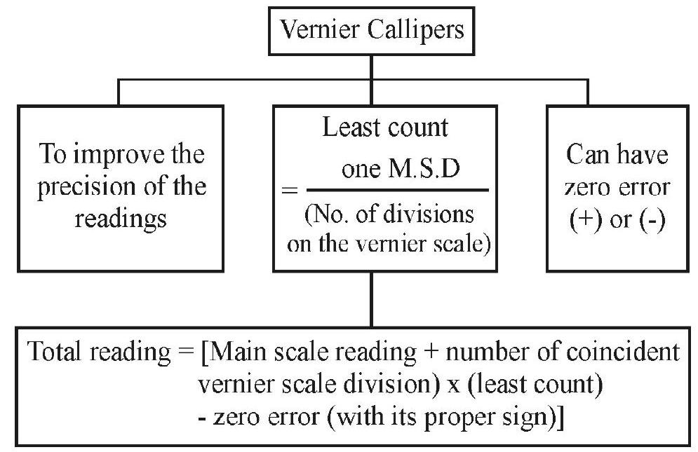
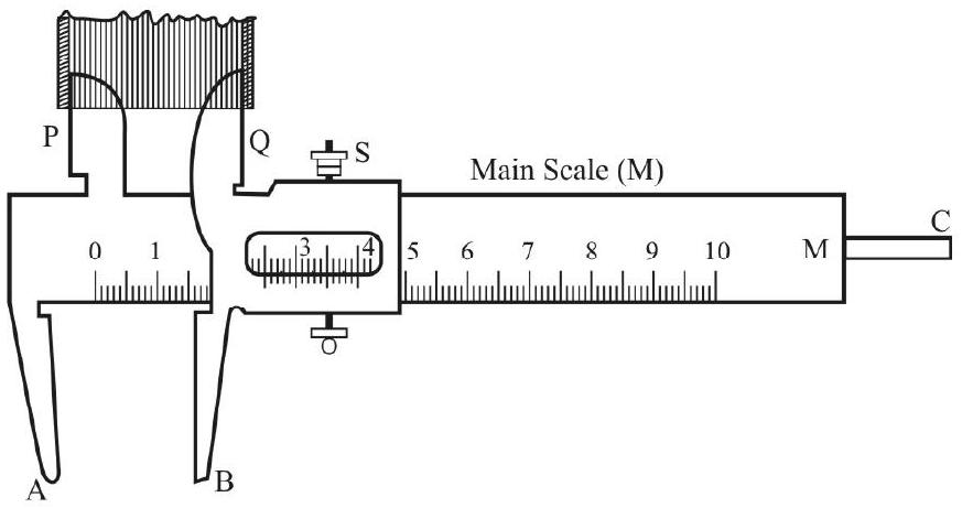
Vernier Callipers
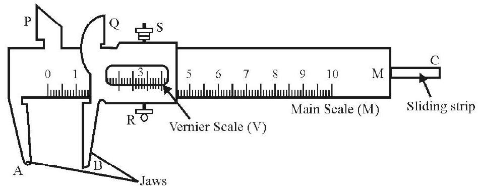
The essential parts of this device, invented by the French mathematician, Pierre Vernier, are shown in the figure below.
Leart Count of the Vernier
The use of an additional scale - called the vernier scale - enables this device to have a much better ’least count’ than the metre scale. The least count of a vernier callipers is given by the formula:
Least count
Reading the Vernier
The reading of the the vernier is a two step process:
(i) reading the main scale value just before the zero of the vernier scale and
(ii) finding the number (n) of the vernier scale division that just coincides with some main scale division.
The total reading equals
Main scale reading
Thus in the fiture given here
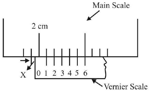
The total reading of the vernier callipers (least count
‘Zero Error’
A given vernier callipers in said to have a ‘zero error’ if the zero of the vernier scale does not coincide with the zero of the main scale when the jaws of the vernier (just) touch each other.
‘Zero error’ can be positive or negative. It is positive when the zero of the vernier lies to the right of the zero of main scale. (when the jaws just touch other).
It is negative when the ‘zero’ of the vernier lies to the left of the zero of the main scale (when the jaws just touch each other). Zero error must always be algebrically subtracted from the observed reading.

It is important to remember that before using a vernier callipers, we
(i) Find / know the value of its one main scale division as well as its ’least count’
(ii) Check for the presence of any ‘zero error’ in it. If a zero error is present, we need to know both its magnitude and sign.
(iii) Always apply the relevant ‘zero correction’ to the readings taken by it.
Using the Vernier
For doing any experiment with the vernier, we first find
(i) its least count and
(ii) zero error, if any, in it.
These have to be used, in the manner already explained, in all readings taken with the vernier.
1. To measure the external diameter of a given spherical object, say, a given cylindrical vessel / glass marble.
After finding the least count and zero error, the given object is held between the ‘jaws’ of the vernier in the manner shown.
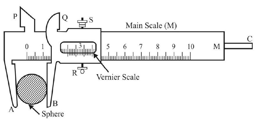
The reading are taken by holding the given object first in one-direction and then in a direction perpendicular to that. These ‘pair of readings’ are repeated at ‘at least three points’ on the object. The ‘zero-correction’, if needed, is applied to the mean of all the redings taken. This mean corrected value (appropriately ‘rounded off’, as per the least count of the given vernier) gives the diameter of the given object.
2. To measure the internal diameter and depth of a given (cylindrical) beaker / calorimeter.
We make use of the upper / outer jaws of the vernier callipers and the sliding strips provided at its back, for taking these readings. The relevant settings are shwon in the figures given below.
The readings, for the internal diamtere, are taken in the same way as those for the ’external diameter’. We again take readings in two mutually perpendicular directions at ‘at least three points’ in the beaker / calorimeter.
The readings for the ‘depth’ may be taken, only once each, at ‘at least three ponits’ within the beaker calorimeter. It is important here to keep the vernier in a vertical position and to keep the edge of the main scale on the mouth of the beaker / calorimeter. The zero correcion, if needed, has to be applied to the mean of the readings taken and the final result ‘rounded off’ as per the least count of the given vernier.

EXPERIMENT-2
Screw Gauge: Its use to determine thickness / diameter of thin sheet / wire.
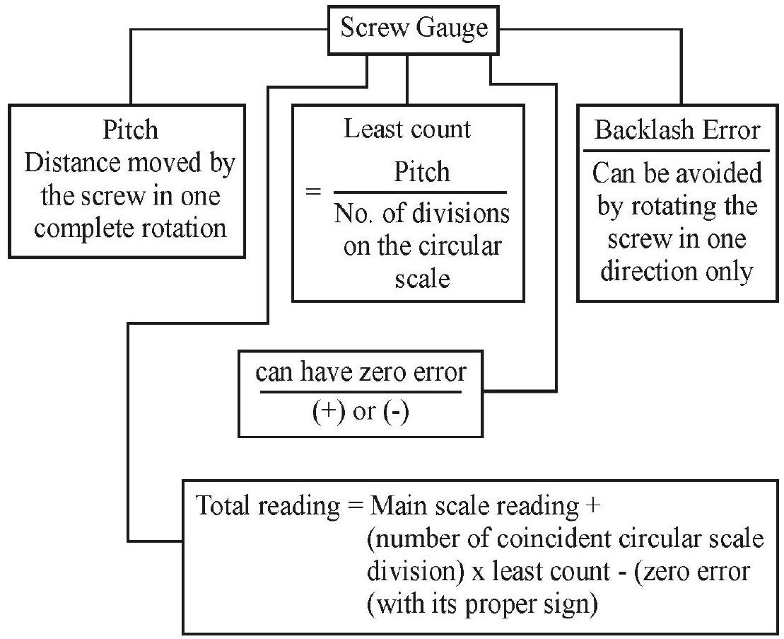
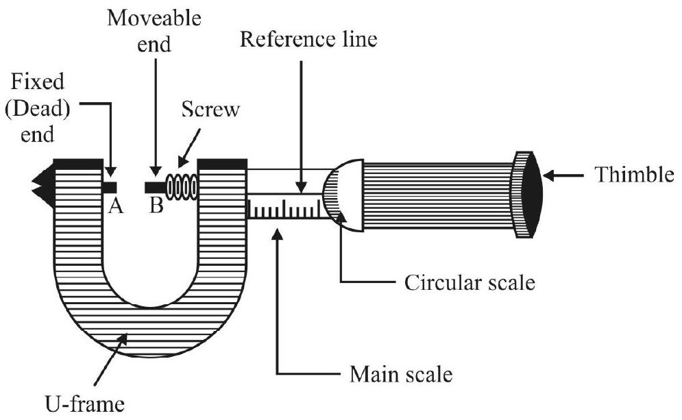
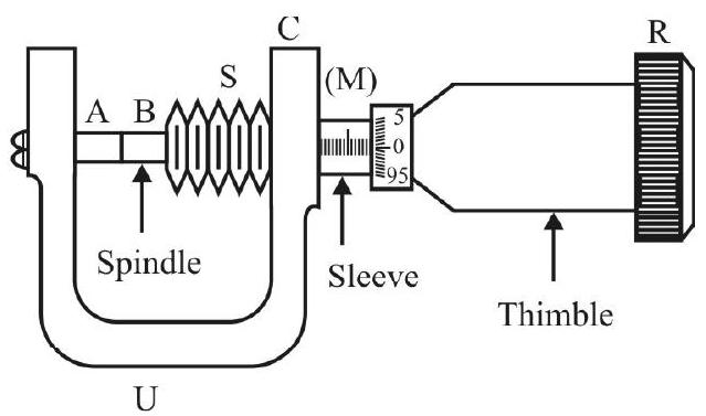
Screw Gauge
A screw gauge - also sometimes known as the micrometer - has an accurately threaded screw having a closely fitting nut. The threadings, of the nut and the screw, match each other. When rotated, the screw not only rotates along a circular path but also advances along a linear path.
The essential parts, of the screw gauge, are shown, and labelled, in the figure given here.
Pitch
The pitch, of a screw gauge, equals the linear distance moved by the screw when it is given one complete rotation. It equals the separation between the successive threads of the screw.
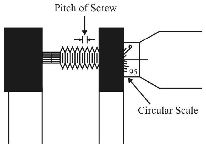
Least Count
The minimum distance, that can be measured by a screw guage, is known as its least count.
The circular scale, in a screw gauge, has (usually) 100 divisions on it. The least count of a screw gauge is therefore, given by
The screw gauges, in common use, have a least count of
Reading the Screw Guage
The (thin) sheet / wire, whose thickness / diameter is to be measured, is ‘just held’ between the faces of the (fixed) and A and the (movable) and B of the screw gauge. At this position, the reading of the main scale (say m), just before the end of its circular scale, is read. One also notes the number (n) of the circular scale division that just coincides with the line of graduation of its main scale. The total reading, of the screw gauge, is then
Totao reading
Zero Error
Due to wear and tear, or due to some manufacturing defect, the screw gauge can have a zero error.
When the faces of the ends A and B of a screw gauge are put just in contact with each other, and the zero of the circular scale lies along the line of graduation of the main scale, the screw aguge does not have any zero error. This is shown in the figure below.
Quite often, however, the perfect, or ideal condition shown above, does not hold. The ‘zero’, of the circular scale, may lie below / above the ‘reference line’ (the line of graduation of the main scale) when the faces, of the ends A and B, are just in contact. When the ‘zero’, lies below the reference line, the screw gauge is said to have a positive zero error. Whe, the ‘zero’ lies above the reference line, the screw gauge is said to have a negative zero error.
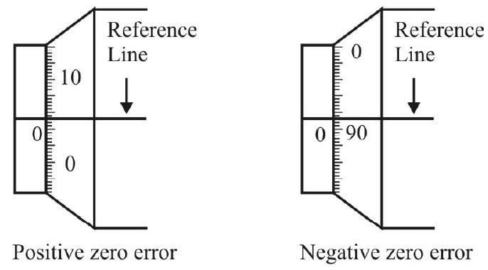
The magnitude, of the zero error, equals the product of the least count (of the screw gauge) with the number (with reference to its zero) of circular scale division that coincides with the reference line. Thus in the figures above, the magnitudes, of the zero error, are
The zero error is always subtracted algebraically from the observed readings.
Backlash Error
The ‘wear and tear’, present in an ‘in-use’ screw gauge, can bring in some ‘play’ in the motion of its screw. In such cases, the screw may not move forward even when the screw head is being rotated. This error is known as ‘backlash error’.
It can be avoided / minimized by always rotating the screw in one direction only.
EXPERIMENT-3
Simple Pendulum: Dissipation of energy by plotting a graph between square of amplitude and time.
CONCEPT MAP
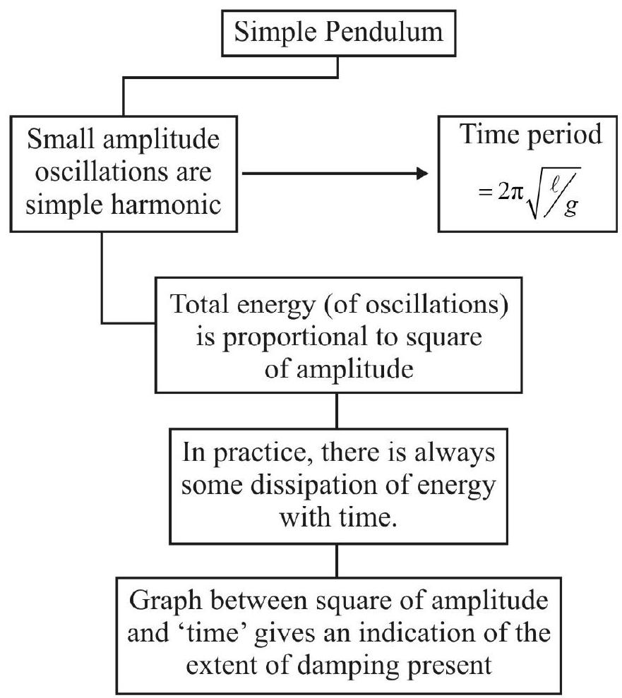
Simple Penculum
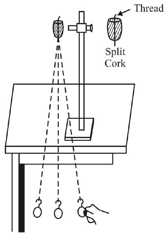
An ‘ideal’ simple pendulum has a ‘point’ mass, suspended from a weightless, inextensible string.
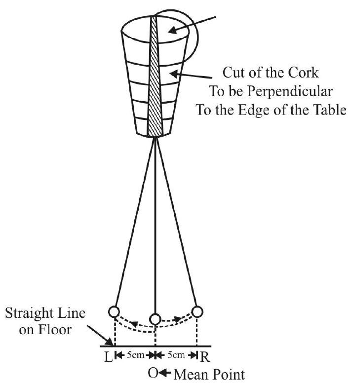
In practice, it is a good quality sewing thread that usually serves the purpose of a ‘weightless’, inextensible string. The ‘point mass’ is usually a small heavy metal sphere (known as the bob) that has a hook for attaching it to the thread. The other end of this thread is put in the cut of a split cork; this cork is firmly held in a suitable stand.
We take the distance between the point of suspension, and the centre of mass of the bobo, as the ’length’ of a given simple pendulum.
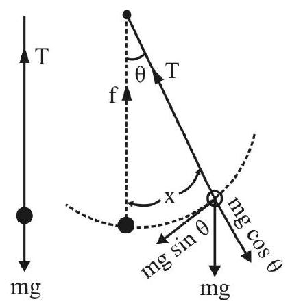
Nature of Motion of a Simple Pendulum
The bob, of a simple pendulum, oscillates in a ‘periodic way’ when it is displaced to one side (from its normal equilibrium position) and ’let-go’. These periodic oscillations are (very nearly) simple harmonic oscillatinos only if the initial displacement (the amplitude) of the bob (from its equilibrium position) is quite small in comparision to the length of the simple pendulum. This can be seen as follows:
The equation of motion, of the angular oscillations, of the bob, is
or
or
where
If
This is the equation of a simple harmonic motion of time period,
Energy of a Particle Executing SHM
The displacement, of a particle, executing SHM, is a sinosoidal function of time. If can have the form
The velocity, and accleration, are, therefore, given by
and
The oscillating particle has both K.E. and P.E., at different points, on its oscillation path. These are given by
K.E.
and P.E.
The total energy, having a constant value at all points and at all times, therefore, equals
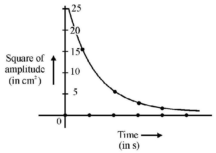
For a pendulum of a given length, the total energy is, thereore, proportional to the square of the amplitude of its oscillations. We may, therefore, take the square of the amplitude, of the oscillations of a given simple pendulum, as an ‘indicator’ of its ’total energy’.
Dissipation of Energy with Time
A practical simple pendulum is never an ideal one; also it (usually) oscillates in air which can be regarded as a (mild) viscous medium. There is, therefore, some dissipation of enregy, by a (freely) oscillating simple pendulum. We observe this through a gradual but progressive decrease in the amplitude of its oscillations. We express this by saying that the (small amplitude) oscillations of a (practical) simple pendulum, (oscillating in air) are damped harmonic oscillations.
Damped Harmonic Oscillations
THe (mistantaneous) damping force, acting on an oscillating particle, is usually taken as proportional to its instantaneous velocity. The equation of motion, of damped oscillations, is, therefore, usually written in the form:
On solving this differential equation, we find that the
(i) Amplitude of oscillations decays exponentially with time:
(ii) The time period of oscillations shows an increase; the exact magnitude of this increase depends on the magnitude of the damping force that comes in play.
The figures, given below, show the difference between undamped and damped oscillations.

Practical ‘Observation’ of the Variation of Amplitude of an Oscillating Simple Pendulum with Time
A simple method, of observing the variation of amplitude, with time, can be as follows. We draw a line on
the floor, below the oscillating bob. We then mark, on this line, points (on both sides) at distances of
Start with an amplitude of
Time Period of the Simple Pendulum
| S. No. | Amplitude | No. of oscillations taken for the amplitude to have this value | Corresponding value of time (in s) |
|---|---|---|---|
| 1 | 0 | 0 | |
| 2 | |||
| 3 | |||
| 4 | |||
| 5 | |||
| 6 | (nearly) zero |
Table for Graph
| S. No. | 1 | 2 | 3 | 4 | 5 | 6 |
|---|---|---|---|---|---|---|
| Square of Amplitude | ||||||
| Time |
— | — | — | — | — | — |
The graph is likely to show an exponential decay of square of amplitude (
EXPERIMENT-4
Meter Scale: Mass of a given object by principle of moments.
CONCEPT MAP
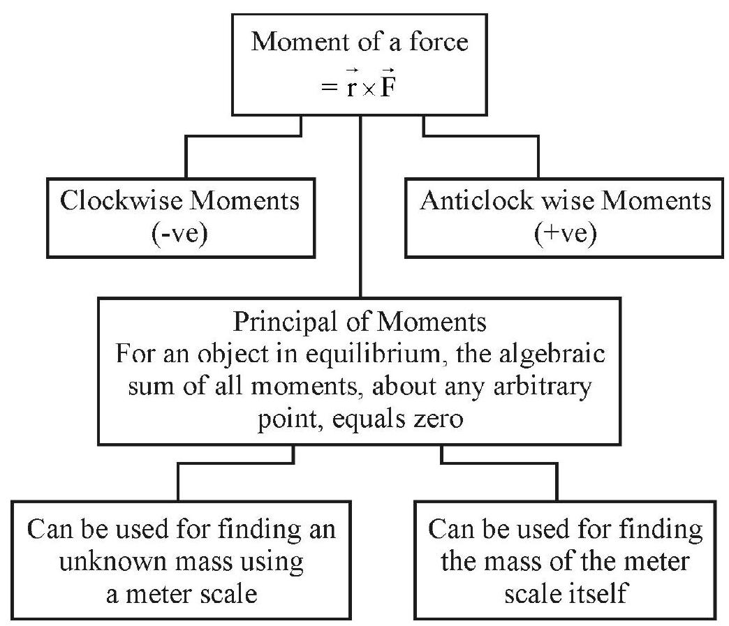
Moment of a Force
The effectiveness of a given force, in producing rotation, of a given object, about some fixed axis (or point), is measured through ’the moment of the given force’, in the given set up.
We define the magnitude of the moment of a force as the product of the magnitude of the force and the ‘force-arm’. Here ‘force-arm’ equals the perpendicular distance between the ’line of action’ of the force and the axis (or point) about which rotation is taking place.
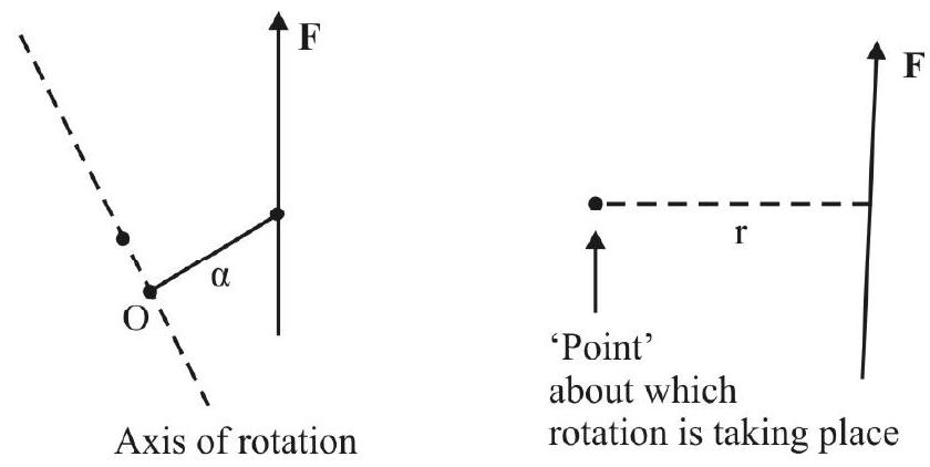
Magnitude of the moment of force
Moment, of a force, (about a given axis or point) is a vector quantity. Its direction is perpendicular to the plane defined by the vector
Here
For rotation about an axis, the origin is taken as the point, where the perpendicular, drawn from the point of application
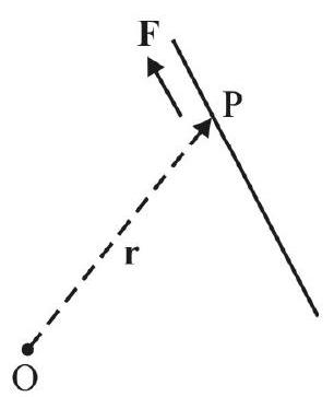
In general, then
Here
Principle of Moments
We state the principle (or law) of moments as follows:
Whenever a body is in equilibrium, under the action of a number of coplanar forces, the sum of the anticlockwise moments, about any arbitrary point, is equal to the sum of the clockwise moments about the same point.
Alternatively, if a body is in equilibrium under the action of a numbe rof coplanar forces, the algebraic sum of all the moments, about any arbitrary point, is zero.
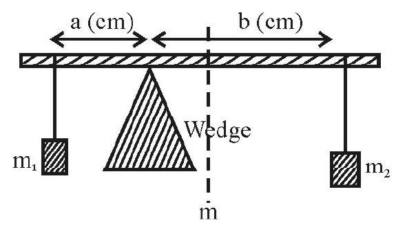
Practicle Application of the Principle of Moments
The principle of moments can be used to find the mass of a given object by using a meter scale, a sharp wedge and suitable known weights. With a slight modification, this ‘set-up’ can be used to find the mass of the meter scale itself.
For finding the (unknown) mass, say
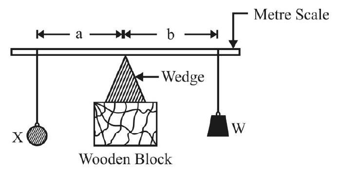
We then have
We may also use a set-up in which two known weights are used. This type of set up is useful when the unknown mass is a heavy mass.
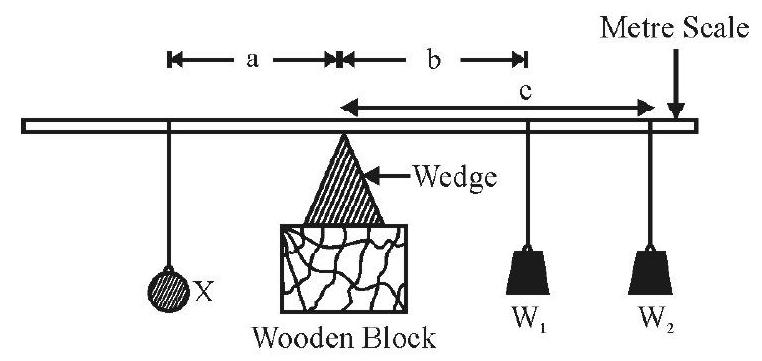
In this case, we have
This set-up can be used to ‘weigh’ the meter scale itself. In this case, the wedge is put at an ‘off-centre’ point and two known masses are put on the two sides of the wedge and adjusted to ‘balance the system’.
In this case, if
When the meter scale is (horizontally) balanced on the wedge (by adjusting) the position of the masses
(Algebraic) sum total of all moments, about the wedge
or
The unknown mass
To use the second ‘set-up’ to find the mass
(Algebraic) sum total of moment of all the weights about the wedge
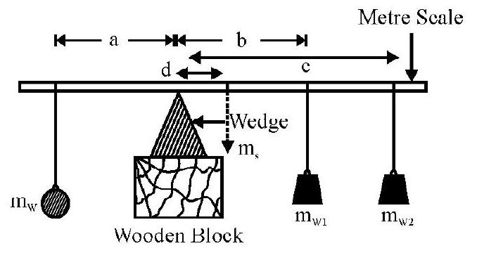
It may be noted that the two ‘weights’,
EXPERIMENT-5
Young’s Modulus of Elasticity of the Material of a Wire.
CONCEPT MAP
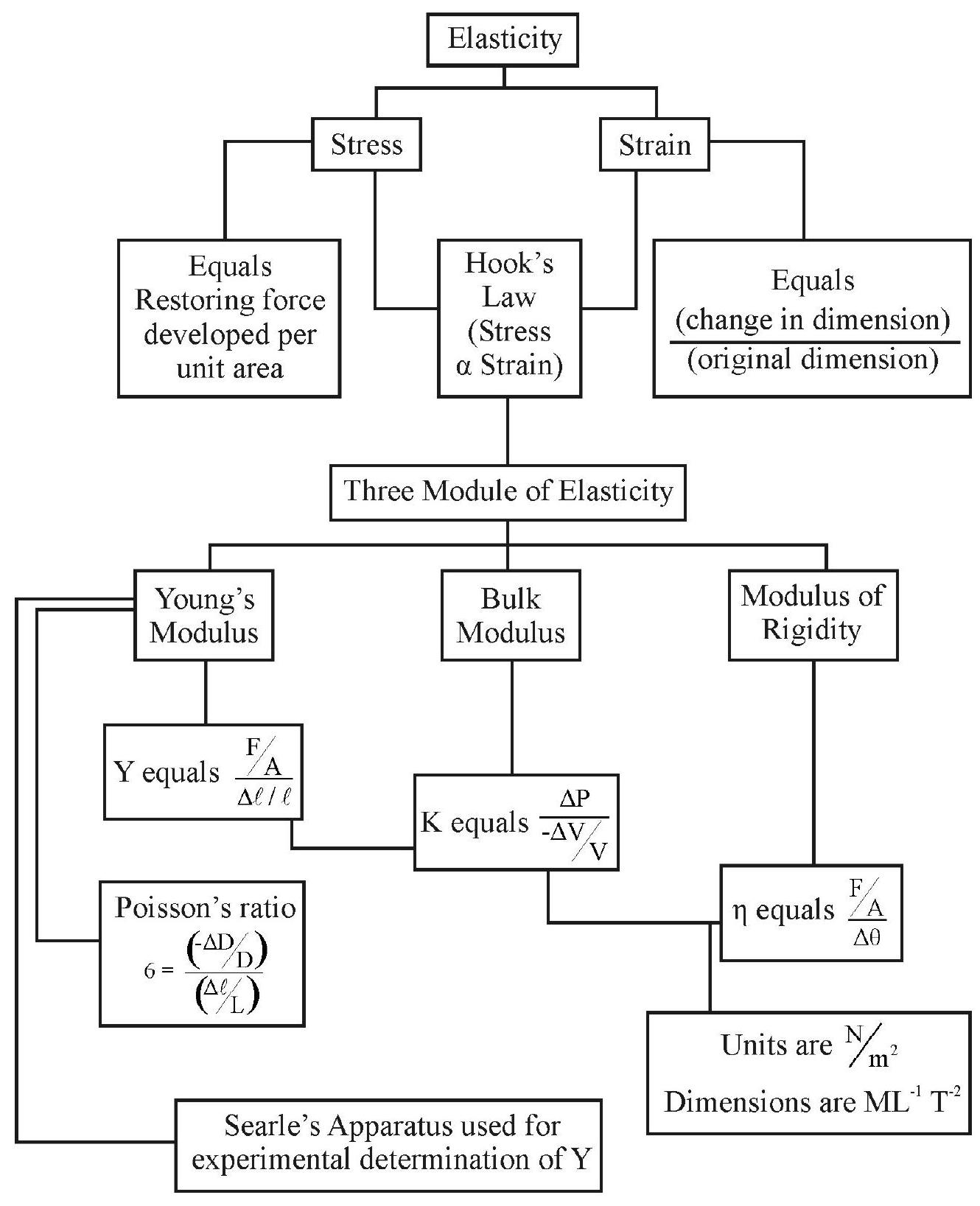
Elasticity
Elasticity is the property of objects of “tending to regain their original conditions after the removal of the deforming forces”.
Stress
When an object is deformed from its normal (equilibrium) condition, internal forces get ‘set-up’ in it that tend to oppose that deformation. This internal recovering force, measured per unit area, is known as the stress developed in the (deformed) object.
The SI units of stress are, therefore,
Strain
When an object is subjected to the action of an external deforming force, the change in the dimensions concerned, measured per unit value of that dimension, is called strain. Strain is a dimensionless quantity; it therefore, has no units associated with it.
Hook’s Law
The fundamental law of elasticity, formulated by Robert Hook, is known as Hook’s law. According to this law:
“For small values of strain, the stress developed in an object, is proportional to the strain produced in it”. The limit, up to which this proportionality between stress and strain holds for a given material, is known as the ’elastic limit’ of that material.
Elastic Module
Within the elastic limits, the stress developed in a material, is proportional to the strain produced in it. Thus, within the elastic limit,
This constant is a characterstic of the material involved and is known as an ’elastic modulus’ of that material.
There are three types of elastic moduli that are defined for a given material. When a material is subjected to a longitudinal strain, the ratio, of the longitudinal stress to the longitudinal strain, is known as the Young’s modulus
In case of a volume strain, the ratio of the volume stress to the volume strain is known as the ‘Bulk Modulus’ of the material. Thus
Sometimes a material is so strained so as to cause a change in its shape without any change in its volume. We then speak of the modulus of rigidity
Modulus of rigidity
The SI units of all these moduli of elasticity is
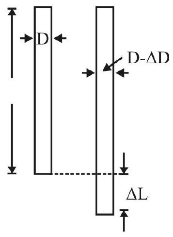
In addition to these three moduli of elasticity, we also define a dimensionless ratio, called Poisson’s ratio
The four elastic ‘constants’,
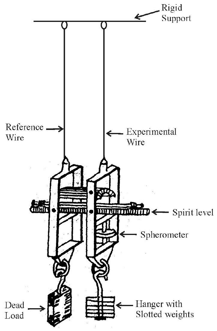
Searle’s Apparatus
Searle’s apparatus is a convenient set up that is often used in laboratory for determining Young’s modulus of the material of a given wire.
A labelled diagram of Searle’s apparatus is given here.
The arrangement, used in this apparatus, to find the (small) change in length of the experimental wire. It has a spirit level, supported horizontally. One end of this spirit level rests on an arm that is fixed to one of the metal frames. Its other end rests on the tip of the screw of a spherometer set-up. The readings of this spherometer, corresponding to the ‘in-centre’ positions of the bubble of the sprit level, without and with the load, on the experimental wire, enable us to find the ‘change in length’ of the experimental wire. These readings, along with readings for the diameter of the wire, enable us to calculate the Young’s modulus for the material of the wire.
Relevant Formula
Let a load
Longitudinal stress
and longitudinal strain
This relation shows that a graph between
EXPERIMENT-6
Surface tension of water by capillary rise and effect of detergents.
CONCEPT MAP
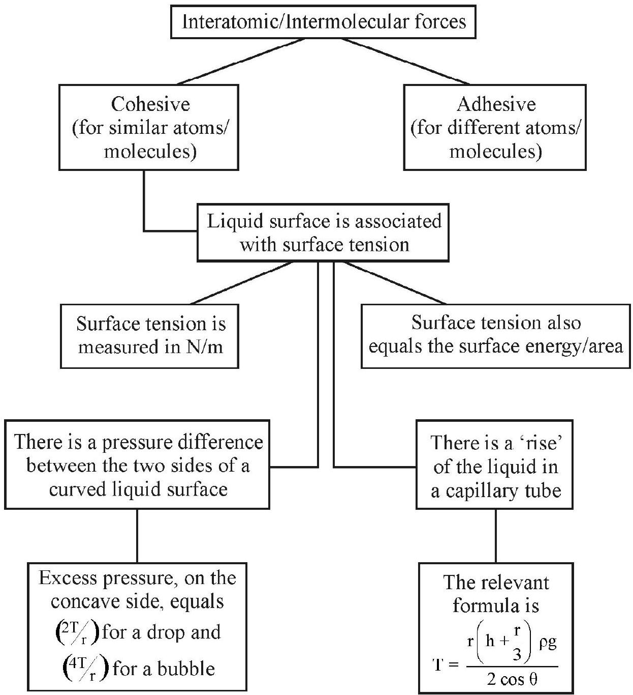
Inter Atomic / Inter Molecular Forces
These are the forces that the atoms/molecules, of a substance, exert on one another. They are short range attractive forces; however, they become repulsive if the atoms / molecules are too close to each other.
Cohesive Forces
Forces, between atoms / molecules, of the same nature, are known as cohesive forces.
Adhesive Forces
Forces, between atoms /molecules of different nature, are known as adhesive forces.
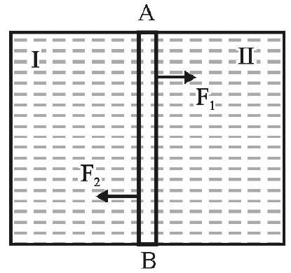
Surface Tension
The surface of a liquid behaves as if it is in a state of stress. The properties, associated with a liquid surface, indicate that each side of the liquid, on either side of an imaginary line on the liquid surface, appears to be pulling the other side towards itself. We call this phenomenon as the phenonmenon of surface tension.
Quantitative Definition of ‘Surface Tension’
Imagine a line, say
The Si units of surface tension are N/m (newton per meter). Its dimensions are
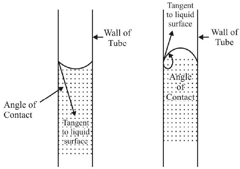
Angle of Contact
The surface of a liquid, when put in a container, acquires a curved shape. The extent and nature, of this ‘curving’, depends on the liquid and the material of the container.
We use a quantity, called ‘angle of contact’, as a measure of the ‘curved meniscus’ of a liquid in a given container. The angle of contact is the angle between the tangents to the liquid surface and the surface of the container. For a concave meniscus (like that of water in a glass tube), this angle is taken as the relevant acute angle while for a convex meniscus (like that of mercury in a glass tube), it is taken as the relevant obtuse angle.
Surface Energy
The potential energy, of the molecules on the surface of a liquid, is more than that of the molecules in its interior. This (extra) potential energy, per unit area of the liquid surface, is known as the surface energy per unit area of the given liquid.
The units of surface energy per unit area, are joule / meter squared
It is easty to see that the surface energy, per unit area of a given liquid, equals the ‘surface tension’ of that liquid.
Pressure Difference Across the Curved Meniscus of a Liquid
The pressure, on the concave side, of the curved meniscus of a liquid, is more thatn that on its other side. It can be shown that this excess pressure, (say
Here
For a bubble, blown out of a given liquid (like say, saop solution), the excess pressure is double that for a liquid drop. This is because, the boundary surface (between) the liquid and air) exists both on the inner as well as the outer side of the bubble.
Thus, excess pressure, inside a bubble, equals

Capillary Tubes
Tubes, of very small diameter (of the order of a mm or so), are known as capillary tubes.
‘Rise’ of Liquid in a Capillary Tube
When a capillary tube is dipped and held vertically, in a container of a given liquid, the level of the liquid, in the capillary tube, is different from its level in the outiside container. This difference, in liquid levels, say h, is related to the surface tension
Here
and
We can take
Quite often
It is this relation that we generally use for finding the surface tension of a liquid by the capillary rise method.
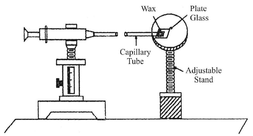
Travelling Microscope
We generally use a ‘special microscope’, called a travelling microscope, for finding the surface tension of a liquid by the capillary rise method. The ‘stands’, attached to the tube of the ‘compound microscope’used here are such taht the tube can be moved both ‘up and down’ (i.e. vertically) as well as ‘right and left’ (i.e., horizontally). There are ‘scales’ (‘main scale’, with its attached vernier scale) that enable one to measure (the horizontal or vertical) movement of the ‘cross wires’ in the ’eye-piece’ of this microscope. The ’least count’ of the vernier, used here, is generally
We use this microscope for measuring the
(i) ‘height’ of ‘rise’, of the liquid in the capillary tube.
(ii) the diameter of the capillary tube.
It is important here to note that
(i) liquids, like water (in a glass tube), ‘rise’ above the ‘outside level’, in a capillary tube.
(ii) liquids, like mercury (in a glass tube), ‘fall’ below the ‘outside level’, in a capillary tube.
Thus ’
‘Experimental Set-up’
A diagram, of the experimental set-up used in the exeperiment for ‘Measuring the surface tension of water, by the capillary rise’ method is given below.
We use this ‘set-up’ for measuing ‘h’ as well as ’
Effect of Detergents
The addition of a deteregent to water, leads to a decrease is the surface tension of water.
Detergents help in cleaning of dirty or greasy clothes. These action can be understand in two ways:
(i) It is energatically favourable to have globs of dirt surounded by detergent and then water.
(ii) The lowering of surface tension, because of the addition of detergents, leads to a better ‘capillary rise’ through the pores in the clothes. This in turn, leads to a better cleaning of the clothes.
EXPERIMENT-7
Coefficient of viscosity, of a given viscous liquid, by measuring terminal velocity of a given spherical body.
CONCEPT MAP
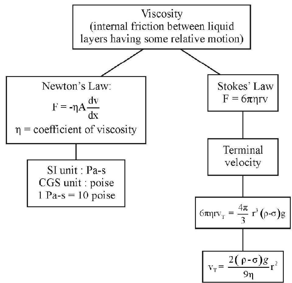
Viscosity
There exists some ‘internal friction’, between adjacent fluid layers, when the fluid is in motion. This ‘internal friction’, which tends to oppose any relative motion between adjacent fluid layers, is called viscosity.
Newton’s Law of Viscous Flow
Let there be two adjacent fluid layers, that are at distances
and
We can, therefore, write
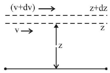
We refer to this result as Newton’s law of viscosity.
Here
Coefficient of Viscosity
From Newton’s law, it follows that
If
We may, therefore, say;
The coefficient of viscosity, of a given fluid, is the (magnitude of) force required to maintain a unit velocity gradient between adjacent layers of unit contact area.
The dimensions of
The cgs unit of
poise
and
It is easy to see that
Stokes’ Law
When an object moves through a viscous fluid, the force of viscosity, that tends to oppose its motion, increases with an increse in its velocity. It was Stokes who obtained a formula for this force of viscosity. The result, obtained by him, is known as Stokes’ law.
According to Stokes’ law:
Here
Stokes’s law can be easily obtained using the method of ‘dimensional analysis’.
Terminal Velocity
Let a (small) object (say, a (small) spherical ball, of radius
‘A Formula’ for ‘Terminal Velocity
Let a (small) spherical ball, of radius
(i) Force of ‘gravity’; this equals the ‘weight’ of the object and is equal to
(ii) Bouyant force, this equals the weight of that volume of the medium that gets displaced by the object;
(iii) Viscous force; as per Stokes’ law this equals
The net (downward) force, acting on the object, is
For
Thus
The slope (say,
We can, therfore, calcualte
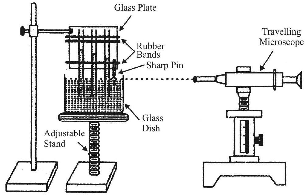
Experimental Set-up
The experimental set-up, used for finding that coefficient of visocisty of a viscous liquid (like glycerine), using (small) steel balls,of different radii, is shown below.
EXPERIMENT-8
Plotting a cooling curve between the temperature of a hot body and time.
CONCEPT MAP
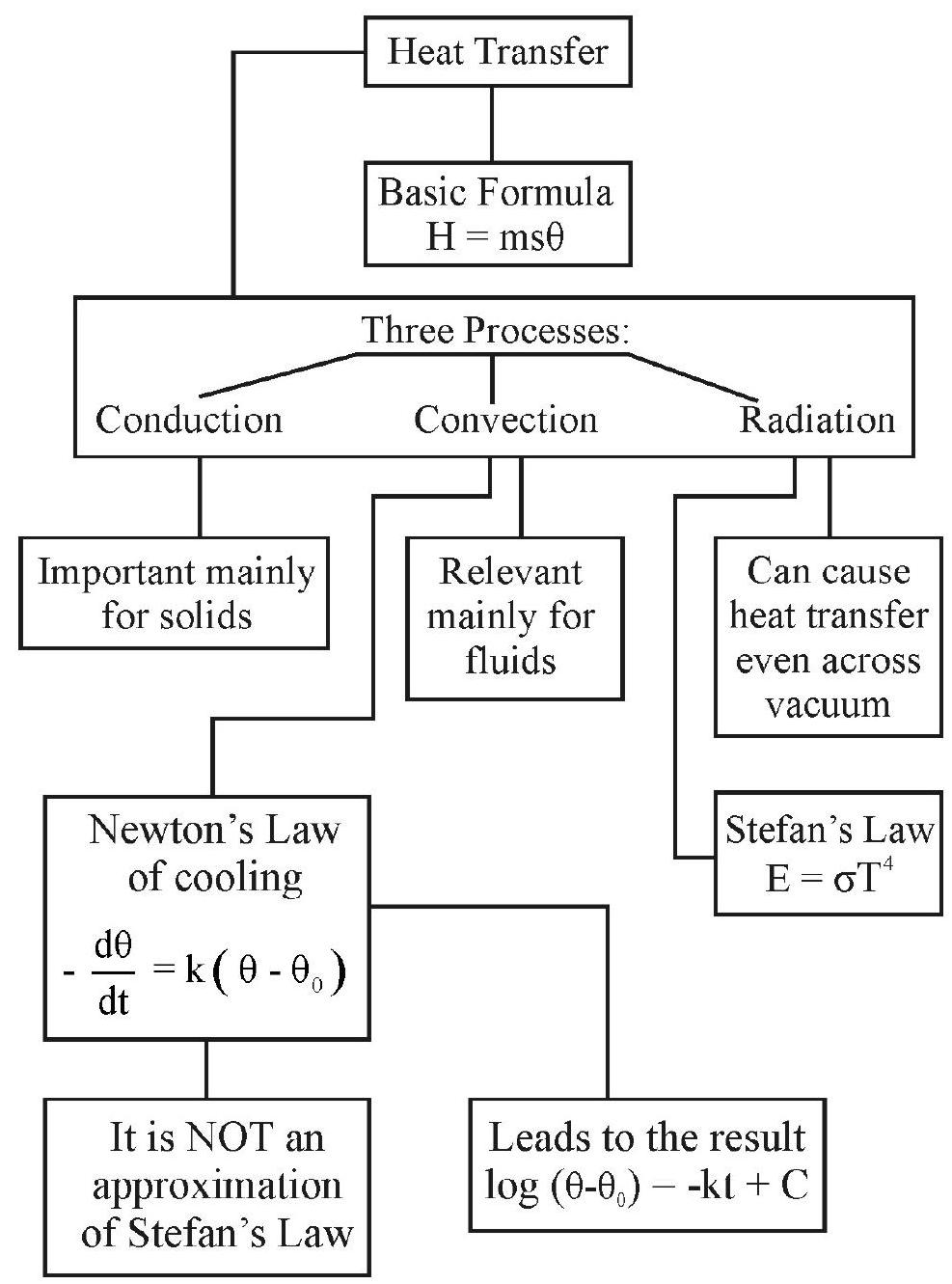
Basic Heat Transfer Formula
The basic formula, for ‘heat transfer’, is
Here
Three Processes of Heat-Transfer
Heat can get transferred, from one object to another, via three processes. There are:
1. Conduction: This is the main method of heat transfer in solids.
2. Convection: This is generally the main method of heat transfer in fluids - liquids and gases.
3. Radiation: This is the process through which heat can get transferred even across vacuum.
Cooling of a Hot Body
When a hot body is kept in ‘isolation’, it cools down by losing heat mainly through convection and rediation. The air, with which it would still be in contact, has very poor conductivity, hence the heat lost by it, through conduction, is almost negligible.
Emission of Heat by Radiation
The law, associated with the ’emission’ of heat by radiation, is Stefan’s law. This law, strictly valid for a perfectly black body, states:
“The heat radiation emitted, per unit area per second, by a perfecly black body, is directly proportional to the fourth power of its absolute (kelvin) temperature”.
In mathematical form:
Here
It may be noted that Stefan’s law is not a ’law of colling’; it is a law that governs the emission of radiation by a black body.
For a ‘black body’, at a temperature
If
Thus, under this approximation
Newton’s Law of Cooling
According to Newton’s law of cooling: “The rate of fall in temperature, of a hot body, is directly proportional to the difference in temperature between the hot body and its surroundings”.
The mathematical form of this law is
This mathematical form leads to the result
or
Thus the time,
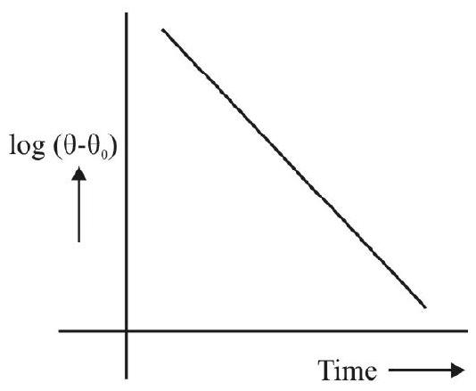
The result
or
tells us that the graph between
If the experimental data leads to such a straight line graph, it may be regarded as verifying Newton’s law of cooling.
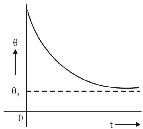
It is often said that Newton’s law of cooling holds only if the difference in temperature, between the hot body and its surroundings, is small. This ‘conclusion’ appears to come from the ‘fact’ that Stefan’s law approaches Newton’s law when the hot body temperature is only slightly above the temperature of its surroundings.
However, the above ‘conclusion’ is not quite correct. This is because, ‘hot bodies’, when kept in air, lose heat mainly through the process of convection. If we aid this process (of loss of heat by convection) by keeping the hot body near an open window, or under a fan, the validity of Newton’s law holds even for quite large difference in temperature between the hot body and its surroundings. Therefore, when we provide such ‘conditions’ in our experiment, the ‘cooling curve’ (temperature versus time graph) has the form shown here and the graph of
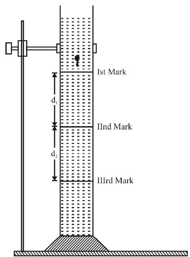
Experiment Set-up
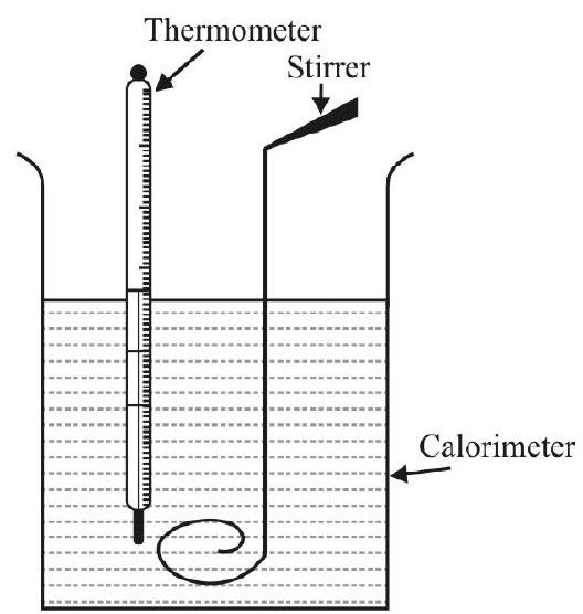
The experimental set-up, for plotting the ‘cooling curve’, may use a calorimeter (without its lid), provided with a stirrer. A thermometer may be suspended in the calorimeter which may be kept near an open window or under a fan. Hot water, pourded into the calorimeter, needs to be constantly stirred and its temperature noted at (appropriate) regular intervals of time. The (temperature) versus (time) graph may then be plotted to get the ‘cooling curve’. One may also plot the
EXPERIMENT-9
Speed of sound, in air, at room temperature, using a resonance tube.
CONCEPT MAP
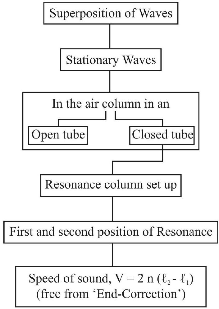
Superposition of Waves
The phenomenon of mixing of two, or more, waves, with one another, to produce a ‘resultant’ wave, is known as the phenomenon of ‘superposition of waves’.
Stationary Wave
The name ‘stationary wave’ is given to the resultant wave that gets formed when two identical waves, propagating in opposite directions, get ‘superposed’ on each other.
The ‘form’ of a stationary wave does not appear to change with time. Such waves are characterised by the presence of
(i) Nodal points (’
(ii) Antinodal points (‘A’ points or antinodes), that are points of maximum disturbance at any given instant oftime.
In a stationary wave, there is always a nodal point between two antinodal points and vice-versa.
Any given antinodal (or nodal) point is separated from its immediate next antinodal (or nodal) point by a distance
Air Columns
We speak of an air column when we have a part of air, confined to definite dimensions, inside a hollow (usually cylindrical) tube.
We refer to such a tube, open at both ends, as an open tube. However, if the tube is closed at one end, it is known as a closed tube.

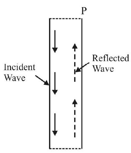
Stationary Waves in an ‘Open Tube’
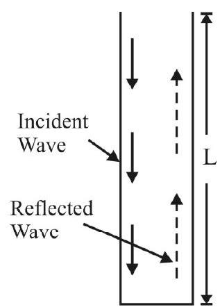
We can get stationary waves in the air column inside an open tube. For this, we need a ‘source’ of waves. When such a source is kept at one end of an open tube, the ‘direct’ waves (sent by the source), and the waves reflected at the other open end, superpose inside the tube and form ‘stationary waves’ in the ‘contained air-column’.
Permissible Modes of Vibration of the Air-column inside an open tube.
The ‘stationary waves’, formed in the air-column in an open tube, have to satisfy the following requirements.
1. The two free ends (or open ends), of the tube must be antinodal points (or antinodes) of the stationary waves formed in the air-column.
2. There must be a nodal point between two antinodal points and vice-versa.
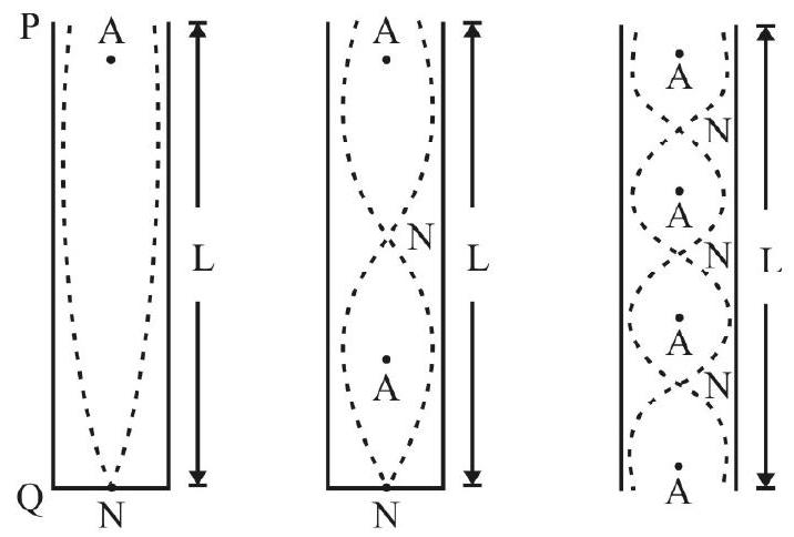
The first three permissible modes of vibration of the air-column inside an open tube are shown below.
We thus obseve that the permissible frequencies of vibration, inside an open tube, can be all integral multiples of the frequency of vibration of its simplest, or fundamental mode of vibration.
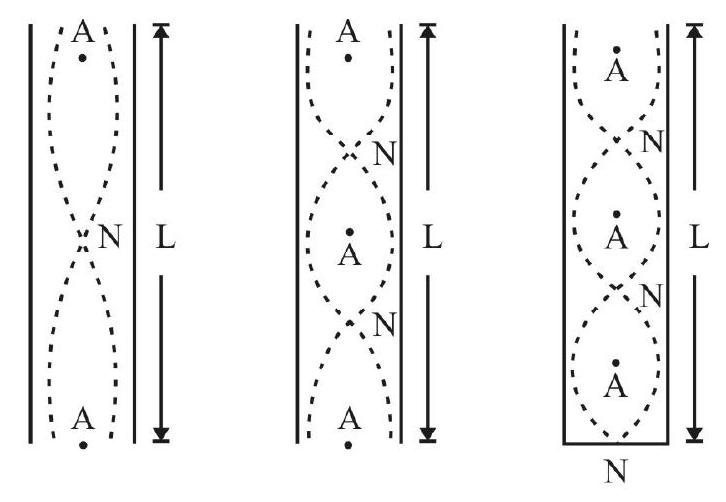
Permissible Modes of Vibration of the Air-column inside a closed tube.
The ‘stationary waves’, formed in the air-column of a ‘closed tube’, have to satisfy the following requirements.
1. The free (or open), of the tube, must be an antinodal point while the closed end must be a nodal point.
2. There must be a nodal point between two antinodal points and vice-versa. The first three permissible modes of vibration of the air-column inside a closed
tube, are shown below.
Here
or
We thus observe that the permissible frequencies of vibration, inside a closed tue, can only be ODD multiples of the simplest, or fundamental, mode of vibration.
The Tuning Fork
The tuning fork is a source of sound that gives out a single pure note of constant frequency. It is, therefore, a standard oscillator of constant frequency.
The shape of the tuning fork is shown below. When it is held from its handle, and one of the its prongs is struck lightly against a rubber pad, the prongs start vibrating transversly, both moving inwards, or outwards, simultaneously. The tuning fork then produces its characterstics note of a constant frequency. The positions of the nodal, and antinodal, points of a vibrating tuning fork, are as shown.

Resonance
The phenomenon of resonance takes place when the frequency of the applied periodic force (used to vibrate a given system) matches the natural frequency of the system itself.
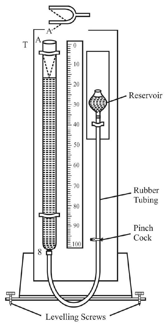
The Resonance Column
The simple set up, used for studying the phenomenon of resonance in a closed tube, has been given the name ‘resonance column’. The length of the air-column, in this set up is adjustable. We adjust the length of this air-column so that its permissible fundamental frequency, or a permissible multiple of that frequency, matches the characterstics (known) frequency of the tuning fork, used to set the air-column into vibrations. The phenomenon of resonance then takes place and one gets a loud, or maximum, sound. A measurement of the length of the air-column, corresponding to which resonance takes place, enables one to calculate the sped of sound in air.
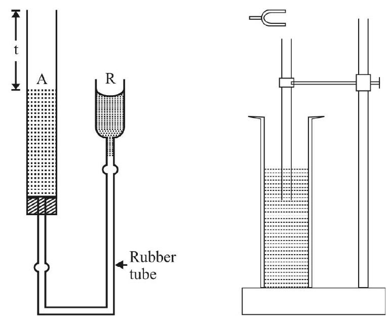
The ‘resonance column’ is available in two simple forms, shown below. However, it is the first form, in which the effective length of the air column is adjusted by raising or lowering of the reservoir, that is used more often.
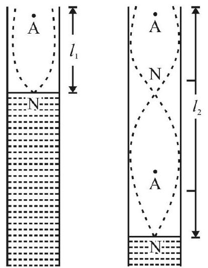
The first and second positions of fresonance, of the air-column in a resonance-column, are shown here.
End-Correction
The reflection of sound does not take place exactly at the open end of the tube. It takes place a little distance (usually denoted by e) above the open end of the tube. This distance ’
Experimental Set-up
The experimental set-up, used in this experiment, is shown below.
Calculation of the Speed of Sound
We take a tuning fork of known frequency (say
and
Now
Hence speed of sound is given by
[Note: We can also calculate the end correction (e). We have from above,
or
Dependence of Speed of Sound on Temperature
The dependence of the speed of sound, (in a gas) on temperature, is as per the formula
This speed of sound (in a gas) varies as the square root of the absolute temperature (of the gas).
EXPERIMENT–10
Specific heat capacity of a given (i) solid, (ii) liquid, by the method of mixtures.
CONCEPT MAP
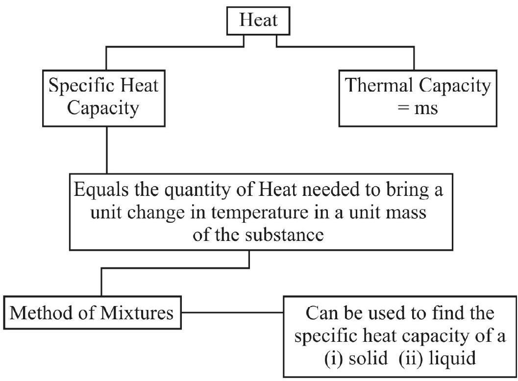
Heat
We may think of heat as a form of energy that gets exchanged between two bodies because of a difference in temperature between them.
The SI unit of heat is, therefore, the same as that of energy, i.e., joule (J)
Quantity of Heat
The amount of heat, gained or lost by a substance, depends on its (i) mass (ii) nature and the (iii) change in its temperature
We, therefore, write the formula:
Here
‘Specific Heat Capacity’
The specific heat capacity of a substance is defined as the quantity of heat needed to bring a unit change in the temperature of a unit mass of the substance. The SI unit of specific heat capacity is
Principle of Calorimetery
Let two bodies, at different temperatures, be brought in contact with each other. The body, at a higher temperature, would then ’lose’ some heat which can be gained by the body at a lower temperature. This process of ‘heat exchange’ continues till the two bodies acquire the same common temperature.
The basic principle of ‘calorimetry’ is that
Heat gained by the ‘cold’ body = Heat lost by the ‘hot’ body.
This principle, therefore, implicity assumes that all the heat transferred remains confined within the two bodies. This is generally not quite true. However, in usual simple experiments on calorimetry, we assume this principle to be a valid principle.
Thermal Capacity or Heat Capacity
The thermal capacity, or heat capacity of a substance, is defined as the quantity of heat needed to change its temperature by a unit amount.
For a substance of mass
Thermal capacity
The SI unit of ’thermal capacity’ is
Calorimeter
The ‘calorimeter’ is the usual simple instrument / device, used in laboratories for experiments on finding ‘specific heat capacity’ and other simple heat related quantities. The following diagram shows the details of construction for a ‘calorimeter’.

Method of Mixtures
In the ‘method of mixtures’ the ‘hot body’ is made to transfer its heat to the ‘cold body’, generally by using a calorimeter. This method is often used for finding the specific heat capacity of a solid as well as a liquid.
‘Specific Heat Capacity’ of a Solid
A calorimeter of known mass (say
A known mass of the solid (say
We then have
Heat lost by the solid
heat gained by the calorimeter and the water / liquid contained in it
Putting heat lost
We can thus calculate the (unknown) specific heat capacity of the solid.
[Note: The use of water / ‘suitable’ liquid, in the calorimeter, depends on the requirement that the given solid should neither dissolve in water / ‘suitable liquid’, nor react chemically with it].
Specific Heat Capacity of a Liquid
Here we can use a (suitable) solid made from a material of known specific heat capacity.
Let
Also let
Also let
We now have
Heat lost by the solid
Heat gained by calorimeter
Heat gained by the liquid
Putting,
Heat gained
We can use this formula to calculate the (unknown) specific heat capacity of the liquid.
[Note: We need to use such a ‘suitable’ solid that neither dissolves in the given liquid nor reacts chemically with it.]
EXPERIMENT-11
Metre Bridge : Determination of resistivity of the material of the given wire.
CONCEPT MAP
Metre Bridge
Aim: To determine the specific resistance, or resistivity, of the material of given wire, using a metre bridge.
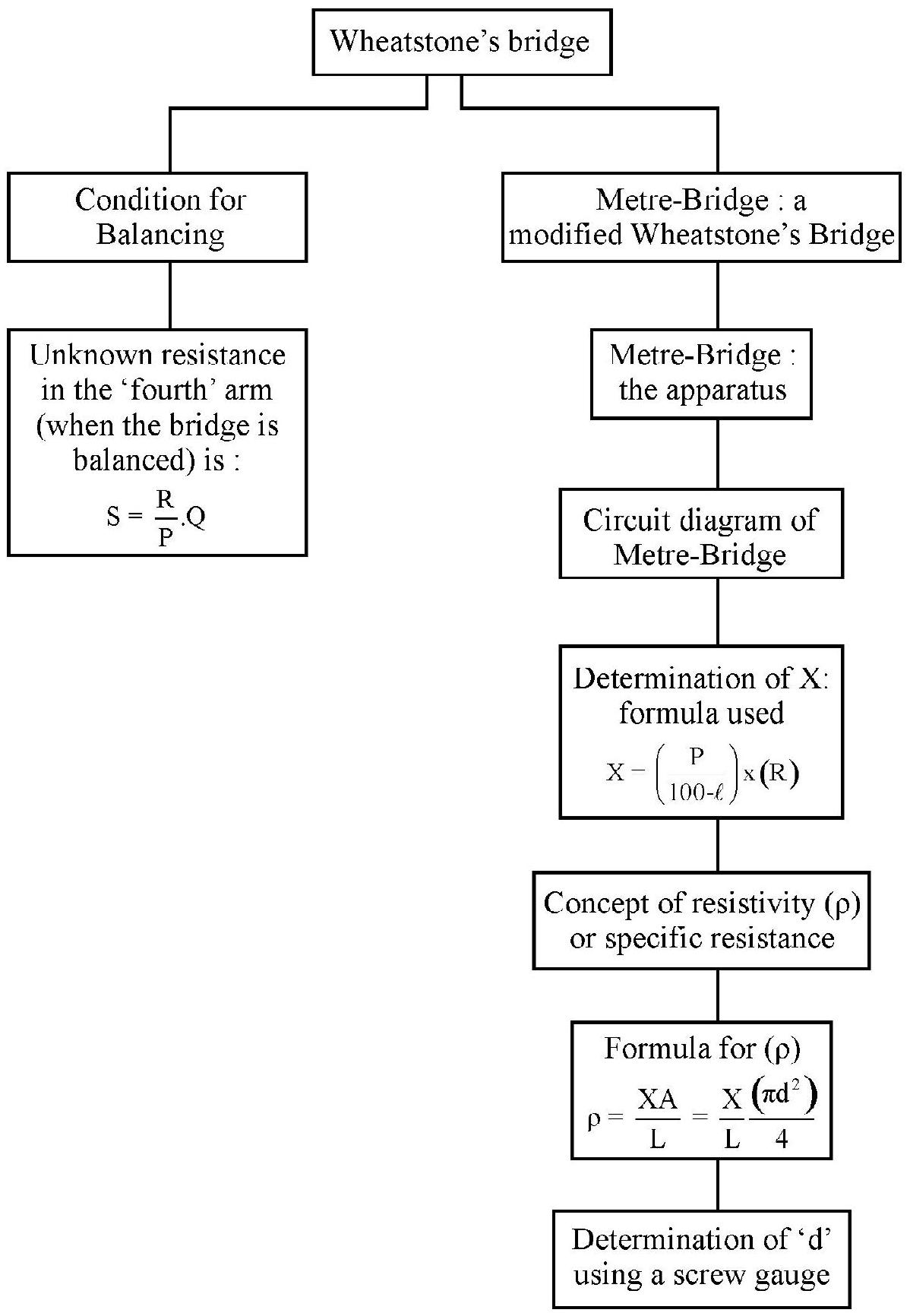
Wheatstone’s Bridge
It is an arrangment of four resistance, say, P, Q, R and S (out of which P, Q and R are known and variable while
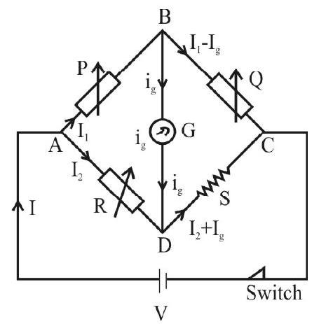
When the circuit is switched on, some current will flow through various branches of the circuit, including the galvanometer (of resistance
Since P, Q and R are known and variable, we can adjust their values to make the current, and thereby the deflection, in the galvanometer reduced to zero.
This process of adjusting the values of
Condition for Balancing of Wheatstone’s Bridge
Applying Kirchoff’s voltage law for the loopABDA, we get:
Similarly, for loop BCDB, we get
When we make
or
and
or
Dividing (3) and (4), we have
This equation
How to Find the value of
From Wheatstone’s condition, we have
where
Metre Bridge, a Modified Wheatstone’s Bridge
Wheatstone’s bridge consists of three known variable resistances, which are usually resisatnce boxes. Handling these individual reisistance boxes, along the unknown resistance wire, is not easy. So a modified bridges has been developed, which is easy to handle and convenient for doing experiments. This is called the metre bridge. The name ‘metre-bridge’ is derived from the use of a one ‘metre’ long uniform wire in this modified bridge.
Metre Bridge: The Apparatus
The metre bridge consists of a uniform resistance wire
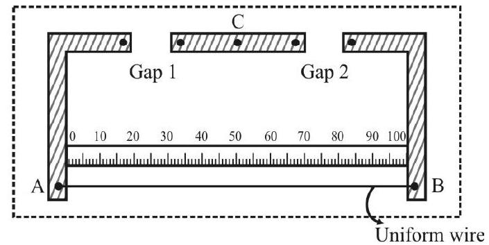
Circuit Diagram of Metre Bridge
The given resistance wire, of unkonwn resistance ’
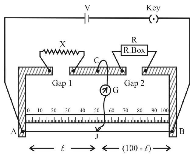
From the terminal at
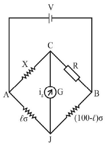
The above circuit of metre bridge is similar to the Wheatstone’s bridge circuit. The related Wheatstone’s bridge circuit is shown for better comparison.
The jockey, pressed on to the uniform wire
Experimental Set-up and Procedure to Find
Using connecting wires, the resistance box, cell key, galvanometer and jockey are connected with the metre bridge as shown is circuit diagram. The given wire (of resistance
The correctness of the circuit is tested by presing the jockey, on to the uniform wire, first near terminal A
and then near terminal B, after the cell key is switched on. If the deflections obtained in the galvanometer are in opposited directions, when the jockey is pressed at
After checking the correctness of the circuit, with R ohm in the resisatnce box, the jockey is pressed near terminal
The balancing length
Determination of
According to condition for balancing of the bridge, we have
As we know the value of R, (taken from the box), and measured value of
A number of observations are to be taken corresponding to
The mean of all the values of
Concept of Specific Resistance or Resistivity (
The resistance, say
(i) the nature of its material
(ii) its length
(iii) its area of cross section (A)
It is found that
In equation (7),
If the conductor is in the form of a thin wire of average diameter (d), then
From equations (7) and (8) we get
Determination of ’
The diameter (d) of the wire, of resistance (X) is measured using a screw guage, following the procedural steps explained in Experiment No. 2,
(Note that
The length ‘L’ of the resistance wire can be measured with the help of a metre-scale.
Once the values of
The following points are considered in order to minizime the error in obtaining thevalue of X, using the metre-bridge.
1. The plug-keys of the resistance box are cleaned using sand paper.
2. All terminals and plug keys are made tight.
3. The circuit is not kept ‘on’ for a long time, as it may cause unnecessary heating.
4. The jockey is not dragged hard along the metre-bridge wire AB, as it may change the crosssectional area of the wire.
5. For better accuracy in the determination of
6. The value of R, put in the resistance box, may be adjusted in such a way that the balancing length
Example-1:
The following data was collected by a student to determine the resistance
| Sl. No. | Resistance in the right gap. |
Balancing length measured from the left gap. |
|---|---|---|
| 1. | 1 | 85.7 |
| 2. | 2 | 74.6 |
| 3. | 3 | 65.8 |
| 4. | 4 | 58.7 |
| 5. | 5 | 53.1 |
| 6. | 6 | 48.2 |
Length of the given wire
Diameter, measured using screw guage is
Show Answer
Solution:
Since the balancing length
The above table can be completed, with the values of
| S1. No. | ||||
|---|---|---|---|---|
| 1. | 1 | 85.7 | 14.3 | 5.99 |
| 2. | 2 | 74.6 | 25.4 | 5.87 |
| 3. | 3 | 65.8 | 34.2 | 5.77 |
| 4. | 4 | 58.7 | 41.3 | 5.68 |
| 5. | 5 | 53.1 | 46.9 | 5.66 |
| 6. | 6 | 48.2 | 51.8 | 5.58 |
Mean
Mean
The formula for
EXPERIMENT-12
Resistance of a given wire using Ohm’s law.
CONCEPT MAP
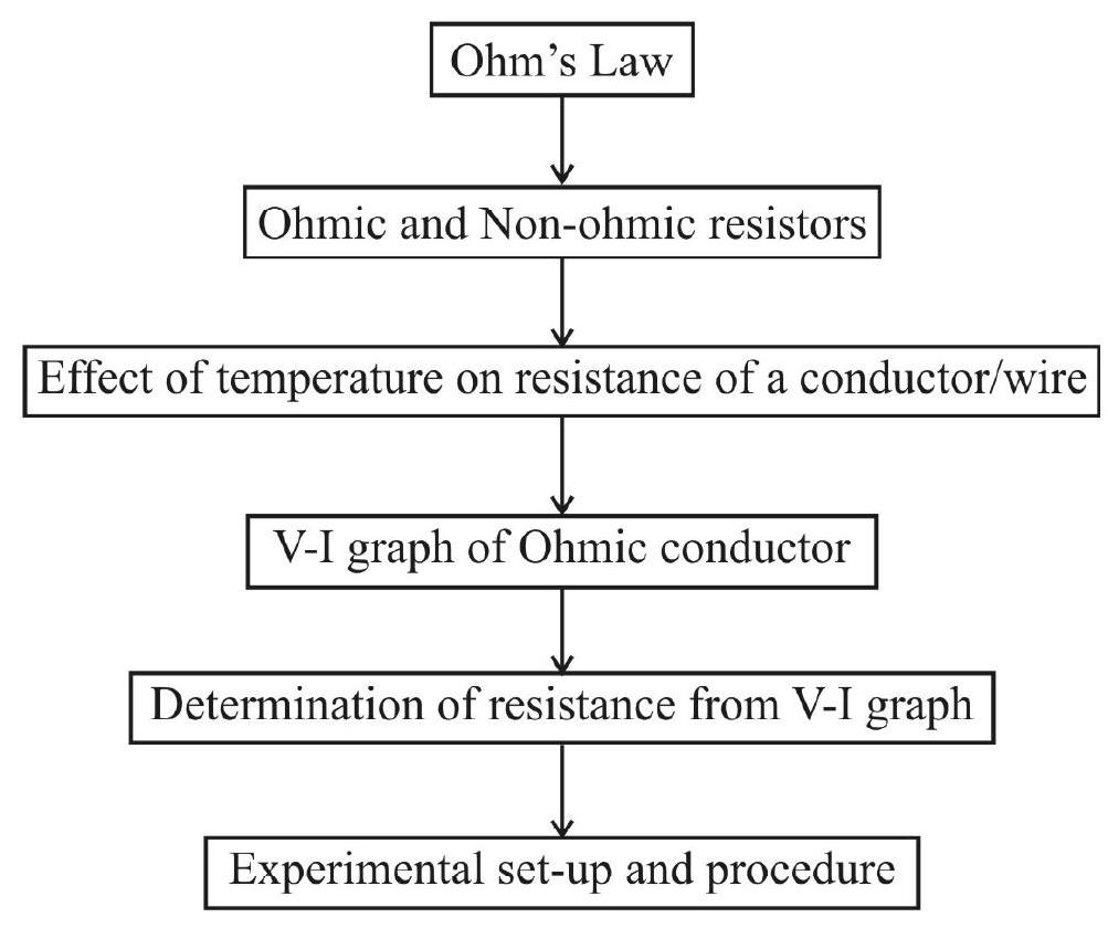
Ohm’s Law
Ohm’s law, for a conductor, states taht the strength of current (I), flowing through that conductor, varies directly as the potential difference (V) applied across its ends, provided all the physical conditions of that conductor, like temperature, length and cross-sectional area, remain unaltered.
That is,
or
where
1. Resistance (R) of a conductor may be regarded as the obstruction offered by the conductor against the flow of charge carriers through it.
2. The cause of resistance is the collision between the moving charge carriers with the atoms / molecules of the conductor as well as with other moving charge carriers.
3. More is the chance of such collisions, more will be the resistance offered.
4. During collisions, energy of the moving charge carriers will be lost to atoms of the conductor. As these atoms / molecules get more energy the conductor, as a whole, will get heated up (or the temperature of the conductor will increase).
5. Thus flowing charges (or current) cause heating effect in the conductor.
6. Resistance (R) of a conductor depends on the following factors:
(i) nature of the conductor
(ii) length of the conductor
and (iii) area of cross-section
7. It is found that:
(i)
and (ii)
or
where
8. The unit of resistance (R) is volt-ampere
9. Since
Ohmic and Non-ohmic Resistors
Materials, which offer resistance, are called resistors.
Ohm’s law is a conditional law, which is valid only when
For them,
Therefore,
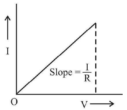
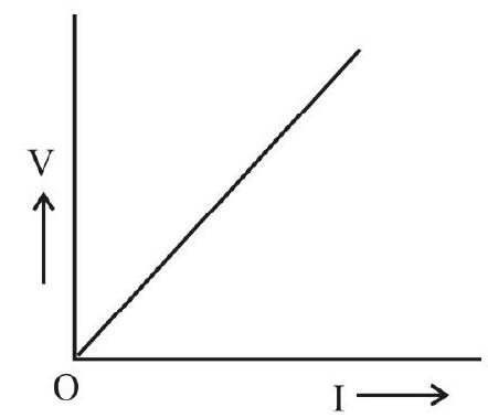
The slope of such a V-I graph will given the resistance (


The slope of I-V graph, therefore, will give the reciprocal of resistance, which is called the conductance
If, for a conductor / resistor, I does not always vary directly as V varies, then V-I graph cannot be a straight line; instead the graph will be a curve. Such conductors / resistors, for which V-I graph is not a straight line, are called non-ohmic resistors / conductors.

- It is to be noted that
- For materials with a positive value of
- For materials with a negative value of
V-I Graph for Ohmic Conductors / Resistors
For ohmic resistors, the value of
This is an ideal situation and in practical situations, it is difficult to obtain such a graph. This is because current I can cause heating of the resistor and thereby change its temperature; this, in turn, can change the value of R.
How to find Resistance from V-I Graph
Let the V-I graph for an ohmic resistor / conductor be as shown below.
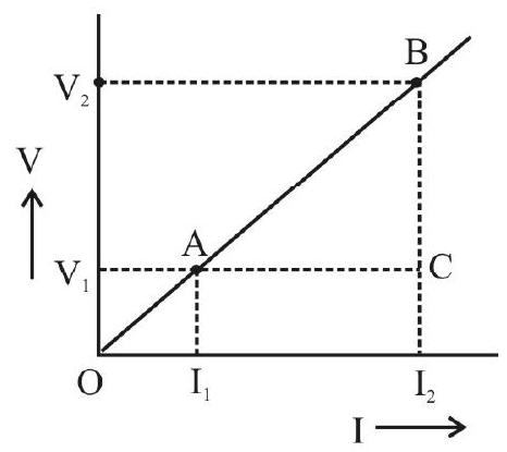
The slope of this graph will be the ratio
(i) Two (quite far apart) points
(ii) Horizontal and verticals are drawn from both points, as shown.
(iii) The right angled triangle
(iv) Slope is calculated as:
(v) The slope gives resistance
Note that, for a perfect ohmic resistor,
In an experimental situation, the values of
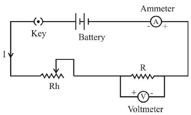
Experimental Set-up and Procedure to Find R
The given resistance wire is connected is series with a current source, a key, a rheostat and an ammeter as shown here. A voltmeter is then connected across the resistance wire.
The rheostat can be adjusted to obtain different values of I. For every value of V (in volt) corresponding value of (in ampere) is measured and recorded. The V-I graph is plotted, with
-
Care should be takes to connect only the very ends of the resistor in the circuit.
-
The least count, and range, of both the ammeter and the voltmeter, are to be recorded for reference.
-
Parallax error must be avoided while taking the readings. The mirror strip, behind the scale of the meters, may be used for this.
-
Heating effect should be reduced by switching off the circuit when not taking the readings.
-
All terminals should be made tight.
EXPERIMENT-13
Potentiometer (i) Comparison of EMF off two primary cells. (ii) Determination of internal resistance of a cell.
CONCEPT MAP
(A)
(B)
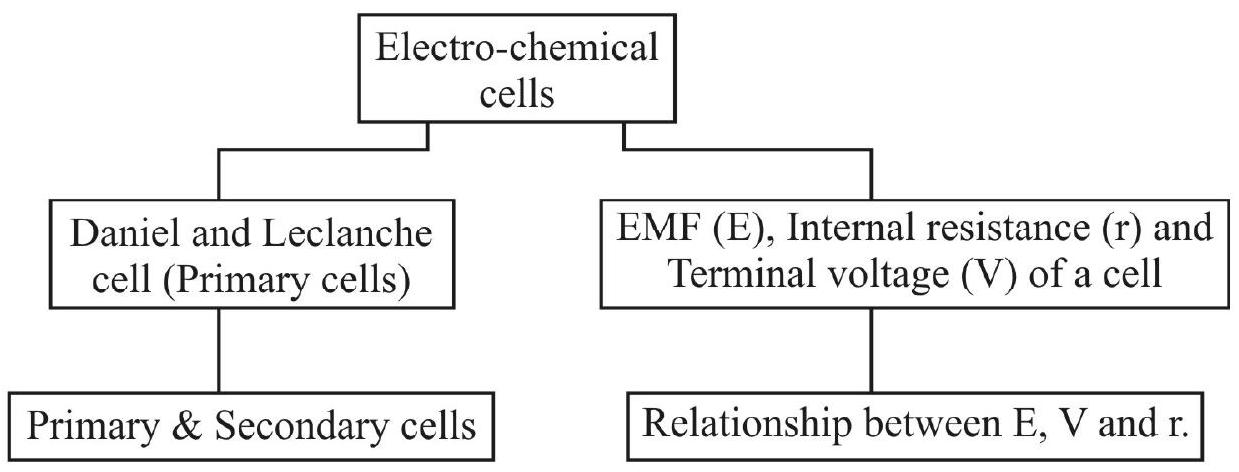
Electro-chemical Cells
These are devices which generate electricity by converting chemical energy to electrical energy by means of chemical reactions.
An electro-chemical cell (simply called a cell) essentially consists of two electrodes, made of two different materials, dipped in a suitable electrolyte (taken in a container / vessel). For example, a simple voltaic cell consists of a copper rod (as positive electrode) and a zinc rod (as negative electrode) which are dipped in dilute sulphuric acid (taken as the electrolyte), taken in a glass beaker, as shown below.
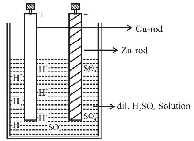
The higher electropositivity of copper will attract
Thus a potential difference gets developed between the two electrodes. When the two electrodes are connected through an external circuit, electrons, deposited on the
During this flow of electrons from
(i) At the Zn-rod
(These two electrons will flow to the copper rod through the external circuit).
(ii) At the
The two
So, for every 2e- flowing through the external circuit one
-
(Note that chemical reactions will begin only when the circuit of the cell is completed).
-
(The
-
The effect of polarisation can be reduced by oxidising hydrogen by using chemicals called ‘depolarisers’.
Daniel Cell and Leclanche Cell
These are electro-chemical cells in which depolarisers reduce the adverse effect of polarisation caused by deposition of hydrogen molecules at their positive electrode.
Daniel Cell
This is a modified simple-voltaic cell.
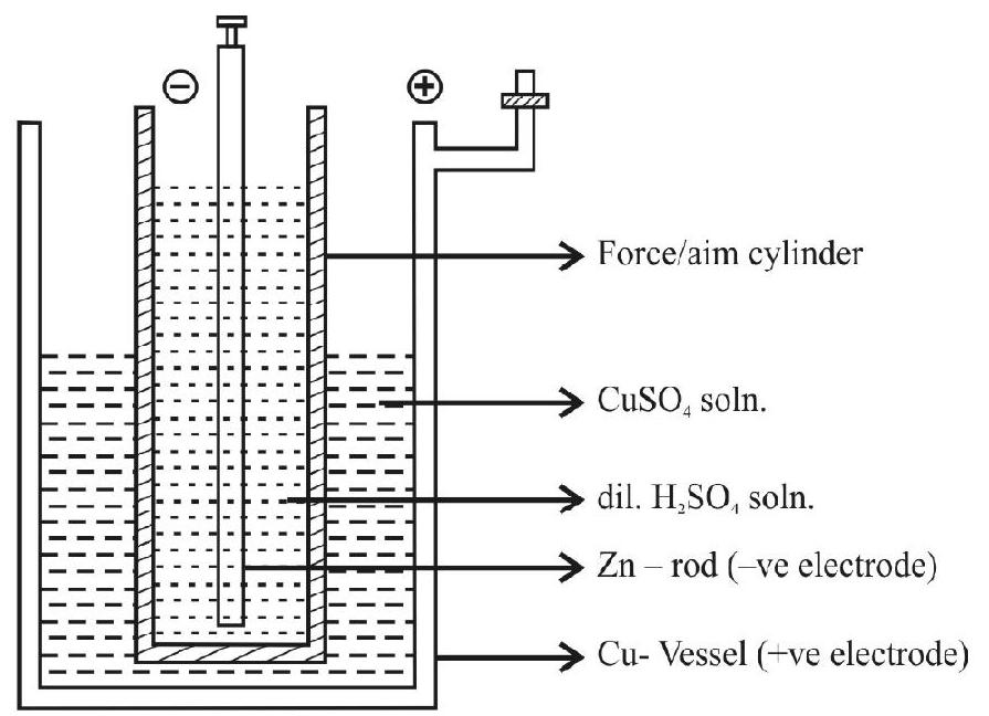
The chemical reactions, which take place at the
(These
The
As
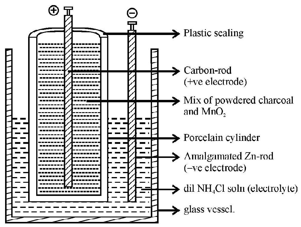
Leclanche Cell
There are two types of Lechanche cell:
(i) Wet Leclanche cell
(ii) Dry Leclanche cell
The “Dry Leclanche cell” is the “Dry cell” which we use commonly in the torches and ‘remotes’. The construction of “Wet Leclanche cell” normally called “Leclanche cell” is shown in the diagram below.
Primary and Secondary Cell
The electro-chemical cells are of two types:
(i) Primary cells
(ii) Secondary cells
Primary cells generate electricity by converting chemical energy into electrical energy. The chemical reactions taking place in primary cells, are irreversible. Hence they cannot be reacharged. Primary cells can not be re-used. Leclanche and Daniel cells are primary cells.
Secondary cells can store electrical energy as chemical energy and this energy gets converted back into electrical energy back when used. The chemical reactions are reversible. These cells can be recharged and therefore, re-used as well. They are also called accummulators as they accummulate energy during charging. Lead-acid accummulators (acid battery) used in automobile cars, invertors etc., are secondary cells.
EMF, Internal Resistance and Terminal Voltage of Cells
EMF refers to electro-motive-force, force which moves electrons. As we know, the force on the electrons cannot be measured directly; we measure the effect of this force in terms of ‘work done’ per unit charge. Every cell (source of electricity) has got an EMF, which depends on the nature of the electrodes used and the electrolyte of the cell.
Definitions of EMF
(i) EMF of a cell is defined as the work done, by the cell, in driving a unit charge through a circuit (closed) once, including the cell.
Hence, EMF is ‘work done’ by the cell per unit of charge.
Therefore, EMF, E
Hence the unit of EMF (E) is also
(ii) The second definition of EMF is in terms of the potential difference. “EMF of a cell is defined as the potential difference between the terminals of the cell, when no current is drawn from it”.
[That is, EMF of a cell is its ’terminal voltage’ when current drawn from it is zero].
Definition of Internal Resistance (r)
It is the resistance offered, by the electrolyte of the cell, against flow of charges (i.e. ions) through it. Internal resistance depends on the following factors:
(i) the temperature of the electrolyte.
(ii) the nature of the electrolyte.
(iii) the concentration of the electrolyte.
(iv) the distance between the electrodes.
(v) the area of the electrodes dipped in the electrolyte.
Definition of Terminal Voltage
Terminal voltage
Terminal voltage always appear across the external resistance, when
(Please note that
Relationship between
Consider a simple circuit consisting of a cell of EMF E and internal resistance
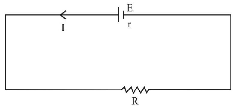
Here, the work done per unit charge, by the cell, is called the EMF.
i.e.
or
Here,
(Remember that: potential difference is equal to work done per unit charge)
But Ohm’s law says that:
Now, the terminal voltage of the cell is same as the voltage across the external resistance, that is equal to
Therefore, from equation (1), we have
Also, the terminal voltage,
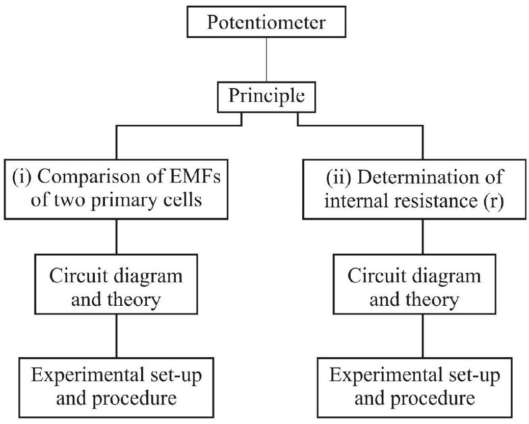
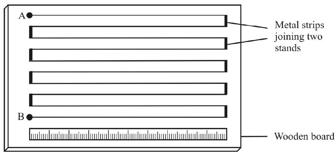
Potentiometer
As the name suggests, it is a device which is used to measure potential difference. Since EMF is also measured as potential difference, a potentiometer can be use to measure EMF also.
A potentiometer essentially consists of a uniform resistance wire, of length from
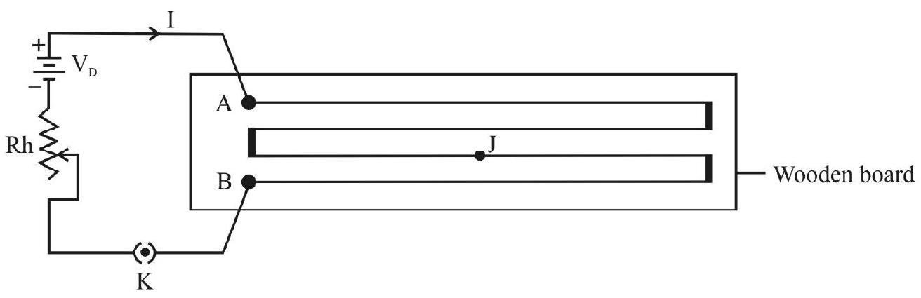
Principle of Potentiometer
Let the resistance per unit length of the potentiometer wire
Suppose the wire AB of the wire is connected to a ‘primary’ circuit, consisting of a driver d.c source (a battery) of voltage
‘Potential drop’ of I
If A is at positive potential, the steady current, I, will produce a potential drop of I
Now if
or
Here,
Thus, we see that
Statement of the Principle of Potentiometer
If states that if a steady current (I) is passed through the uniform wire of the potentiometer (of resistance
Measurement of EMF of a Cell
Consider the potentiometer wire (AB) carrying a steady current (I), driven by the driver cell. Suppose a cell, of EMF (E), be connected to this potentiometer wire through a galvanometer and a jockey, as shown in the figure. (Care should be taken to ensure that positive terminals of both the driver battery and the cell are connected to the terminal A of the potentiometer).
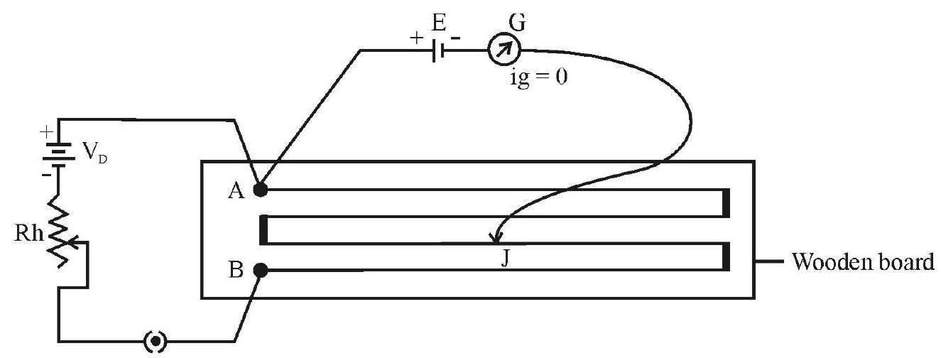
The jockey can be moved the along the wire AB, till the galvanometer shows zero deflection. This is called the balancing of the cell across length
Let
Now, the two potential differences are balanced, in this case. These are:
(i) The potential difference across
length of the potentiometere wire. (i.e.
(ii) The potential difference across the terminals of the cell.
Note that the cell is in a closed circuit here, but the net current drawn from this cell (ofEMF E) is zero (as the galvanometer shows zero deflection) at the balancing position
Therefore, the
or
or
By measuring the value of
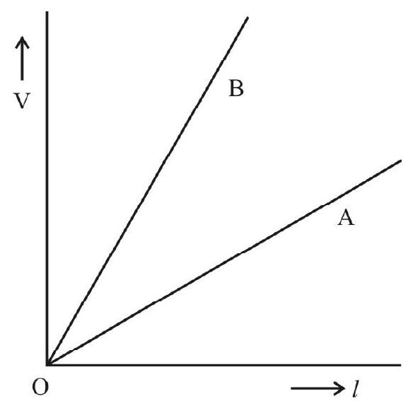
Potential Gradient along the Potentiometer Wire
From the principle of potentiometer, we have,
or
Here
or
It is clear, from equation (4) and (5), that if the value of I is less then the potential gradient will be less. Hence, to obtain the same potential difference
In the adjacent graph,
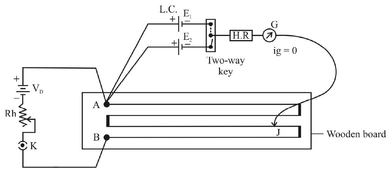
Comparison of EMFs of two primary cells
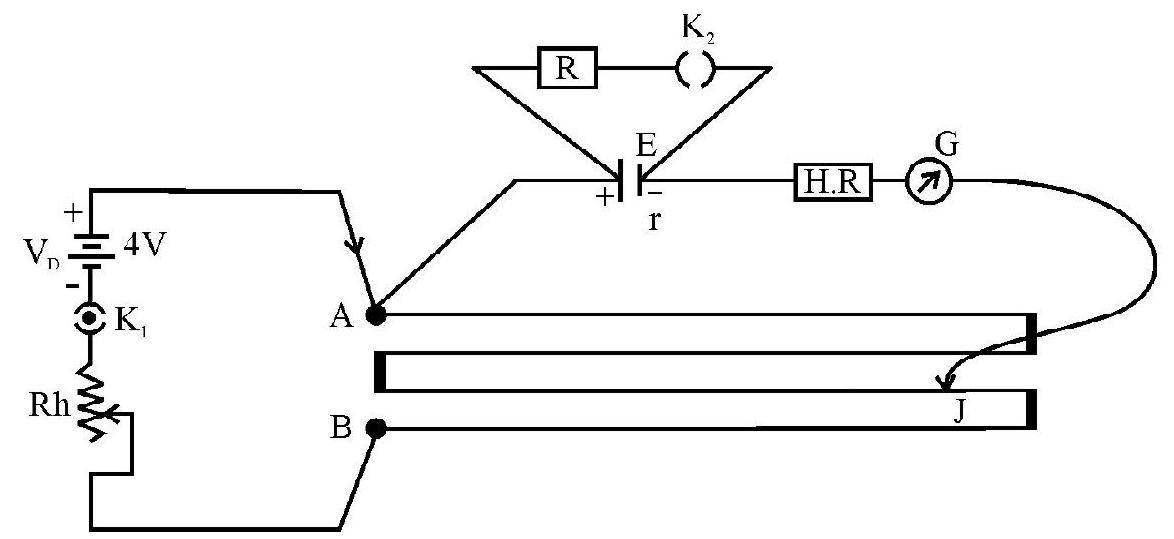
Here, the aim is to compare the emfs of a Laclanche cell
Here, we use:
(a) a potentiometer wire
(b) a primary circuit with a driver cell of voltage
(c) The two cell whose EMFs are to be compared, along with a two-way key, galvanometer, a high resistance (H.R.) and a jockey.
(Note that the H.R. is used to protect the galvanometer from excess current damaging it. The H.R. may be short-circuited to get accurate balancing length).
All the above components are connected as shown in the circuit below.
Formula: It
Experimental Set-up and Procedure
One the circuit is completed as shown in the figure above, the following steps are taken to check the correctness of the circuit.
-
Ensure that all positive terminals (
-
The value of
-
When the Leclanche cell is included in the circuit (as is the case shown in the figure (above), we must obtain opposite deflections, in the galvanometer, when we press the jockey near A, on the wire, and then near B, on the wire.
[If opposite deflections are not obtained the rheostat can be adjusted in order to obtain opposite deflections]
-
Once such opposite deflections are obtained, the circuit set-up is ready for use.
-
Once the circuit is made to give opposite sides deflection, the balancing lengths for lechanche cell (of EMF
-
Let
or
- In order to take more observations, we can change the value of I, by adjusting the rheostat to a slightly different resistance value, keeping two important points in mind:
(a)
(b) opposite deflections are obtained in the case of Lechanche cell in each set of observations.
- The value of high resistance does not affect the balance point position as the observations are taken when
Determination of Internal Resistance (
The objective of the experiment is to determine the resistance offered by the electrolyte of the cell; called the internal resistance (
Since the internal resistance depends on many factors (like the temperature and concentration of the electrolyte, the distance between the electrodes and the surface area of the electrodes dipped in electrolyte), the value of
It is to be noted that, to find
Remember that, in the formula

Circuit Diagram and Formula
Here we use:
(a) A potentiometer wire
(b) A driver circuit consisting of a battery of voltage
(c) A primary cell (say, a Leclanche cell), of EMF ’
(d) A resistance box, in which a known and variable resistance
The complete circuit is shown below.
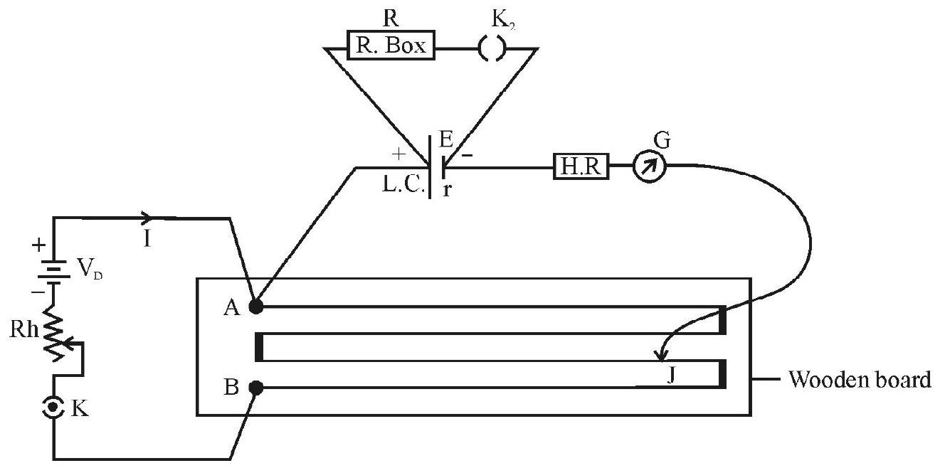
Theory and Procedure
Suppose key
Here, let I be the steady current flowing through the potentiometer wire
Suppose next, a resistance
Now, if
Therefore
We have the formula for
Knowing
The observations can be repeated for various values of ’
[Note that for a set of observations of
The following precautions may be taken to reduce the error in the observations while using a potentiometer.
-
Balancing length
-
Overheating should be avoided by switching off the circuit immediately after every observation.
-
All terminals should be made tight.
-
The jockey should not be dragged hard along the potentiometer wire to avoid any change in the cross-sectional area of the wire.
Example:
The following circuit was used by a student to determine the internal resistance of a Leclanch cell.
The rheostat was kept at the same position throughout and
| Sr. No. | Balancing when |
Balancing when |
|
|---|---|---|---|
| 1. | 10 | 824.5 | 446.0 |
| 2. | 15 | 824.5 | 456.0 |
| 3. | 20 | 824.5 | 496.0 |
| 4. | 25 | 824.5 | 557.0 |
| 5. | 30 | 824.5 | 585.0 |
| 6. | 35 | 824.5 | 591.0 |
Show Answer
Solution:
The formula for determination of internal resistance, using potentiometer, is:
Using this formula the calculated value of
| Sr. No. | ||||
|---|---|---|---|---|
| 1. | 10 | 824.5 | 446.0 | 8.5 |
| 2. | 15 | 824.5 | 456.0 | 12.1 |
| 3. | 20 | 824.5 | 496.0 | 13.2 |
| 4. | 25 | 824.5 | 557.0 | 12.0 |
| 5. | 30 | 824.5 | 585.0 | 12.3 |
| 6. | 35 | 824.5 | 591.0 | 13.8 |
Here, the minimum value of
EXPERIMENT–14
Aim: To determine the resistance
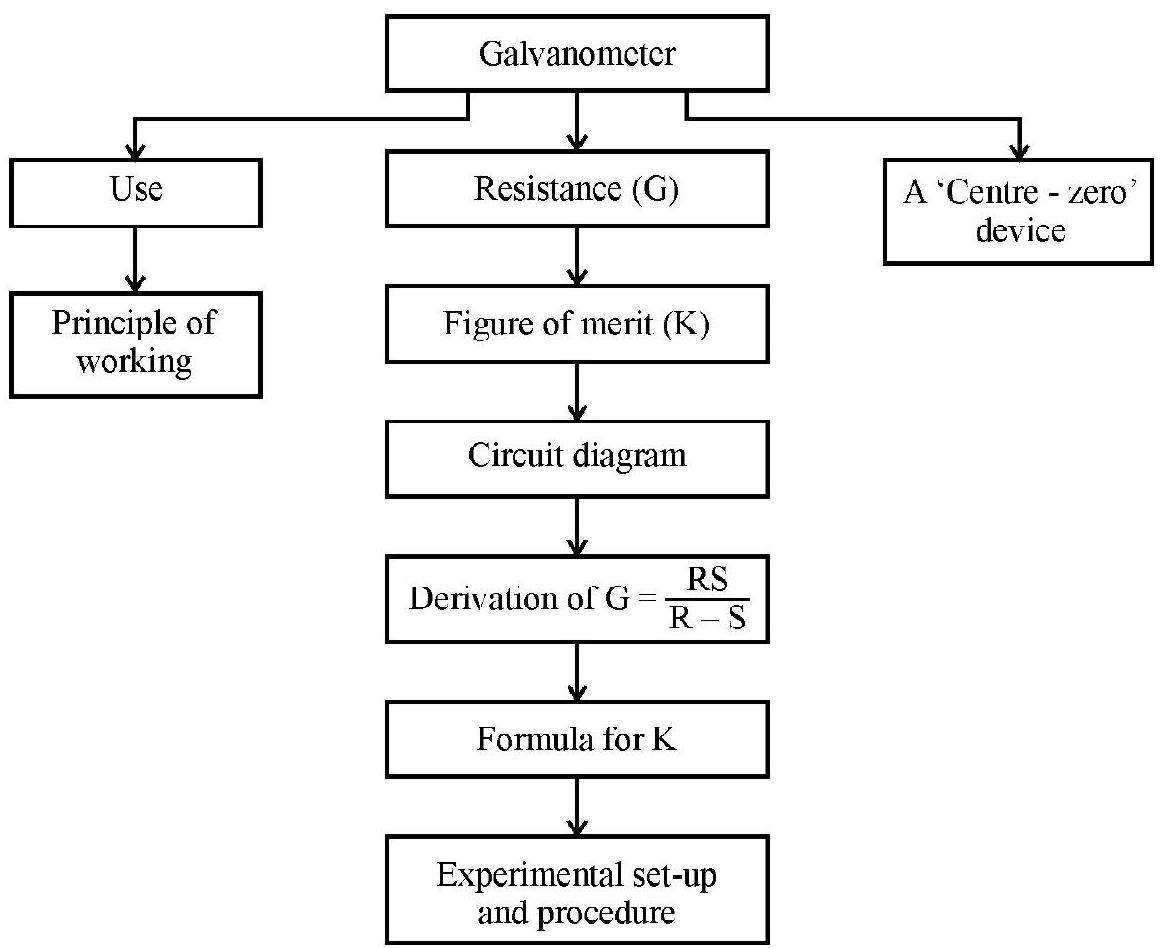
Galvanometer
It is device used to detect very small currents flowing in a circuit.A galvanometer is a very sensitive device.
Principle of Working of Galvanometer
It is based on the principle that a coil, suspended or pivoted in a uniform magnetic field, will experience a torque whe a current (I) is passed through the coil.The extent of its rotation, against an (internal) restoring torque, will be proportional to the current strength. The extent of rotation can be measured with the help of a pointer, attached to the coil, when the pointer deflects and moves over a scale, graduated in divisions. The scale is a linear scale and the pointer is made to coincide with the zero of the scale (when no current is flowing) which is marked at the centre of the scale. This centre-zero scale enable us to observe the direction of current also as the pointer can deflect in both the directions from its zero position (which is at the middle of the scale).
Resistance (G) of the Galvanometer
The coil of the galvanometer is made of a long thin insulated copper wire wound on a rectangular metallic non-magnetic light frame. Since the wire is very thin and long, the wire provides resistance, even though
the wire is made of copper. This resistance, provided by the coil, is called the resistance (G) of the galvanometer. The value of G ranges from around
Figure of Marit (k)
It gives an idea of how sensitive the galvanometer is detecting current. Figure of merit (
That is
If
Since the galvanometer is very sensitive,
(Note that this current is very small and only in
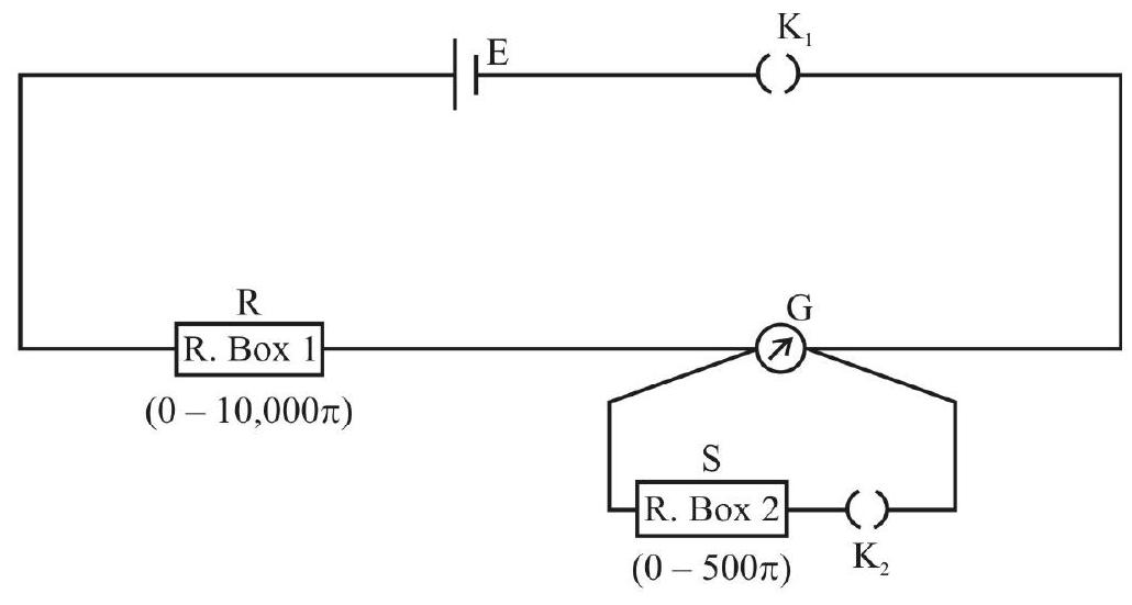
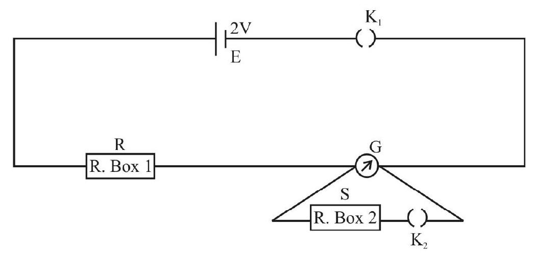
Circuit Diagram
The circuit diagram, used for the determination of G, consists of a d.c source of emf E, a series variable resistance
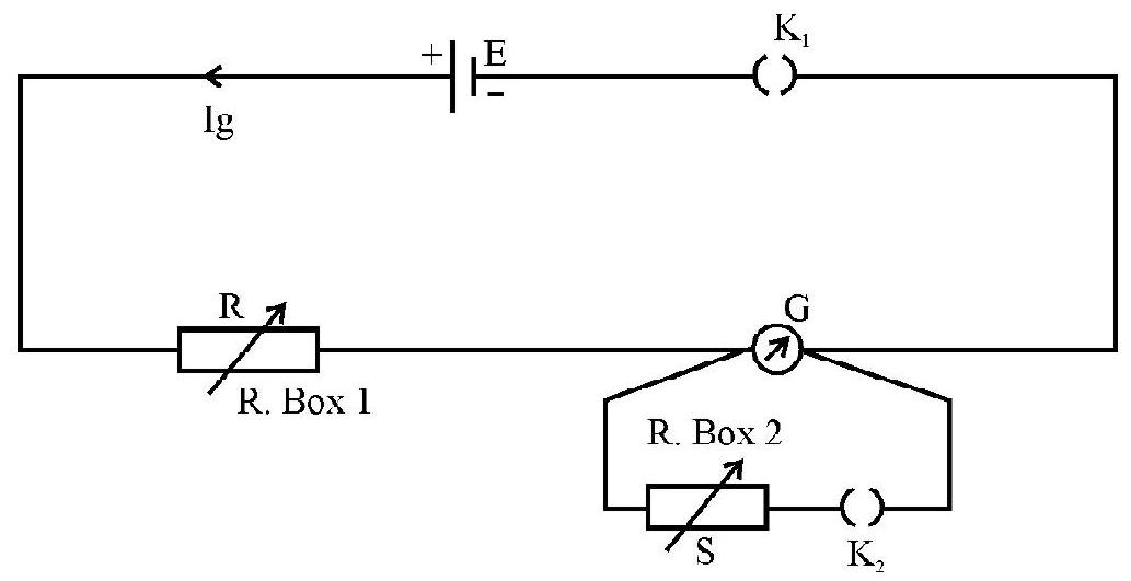
Derivation of the Formula for
Let
or
Now, suppose
Let the current through the galvanometer, now, be
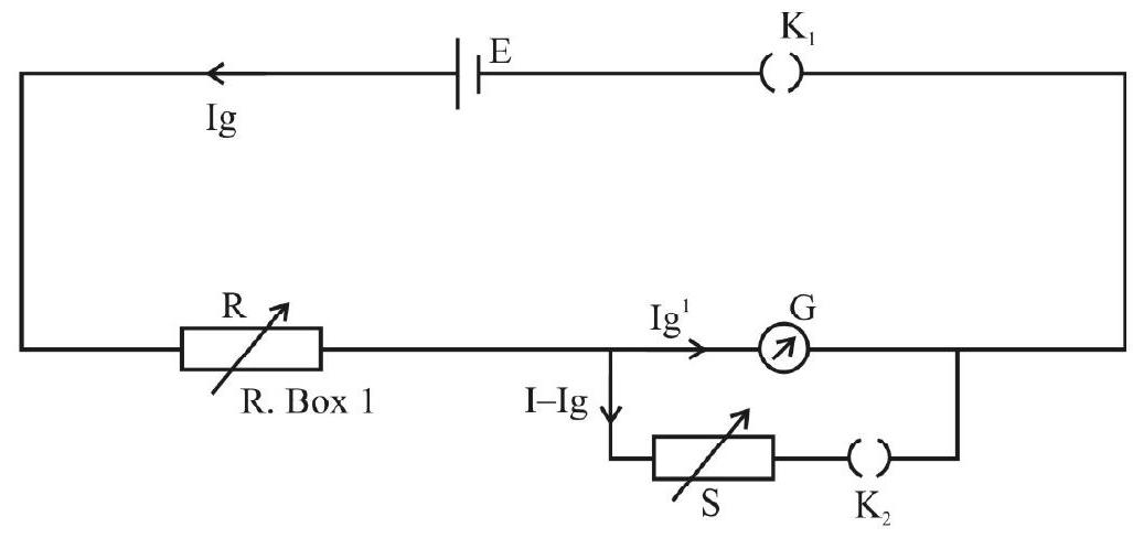
From the parallel connection of G and S,
We have
Also,
The combined resistance with circuit, now is
or
Substituting this value of I in equation(2), we get
or
or
Dividing equation (1) by equation (3), we have
or
or
or
Since
Formula for
From equation (1), we can find the value of
Experimental Set-up and Procedure
A resistance box (1) of range (
Normally, a galvanometer with 30 divisions on its scale, on either side of the zero at the centre, is used in the experiment.
To determine ’
-
Take out a high resistance of
-
Close
-
By suitably adjusting the value of
-
Now
-
Using the value of
-
Observations can be repeated for
-
The mean value
-
Once the value of
Here,
The following precuations may be observed, in order to reduce the error in the observations.
-
The plug keys of the resistance boxes should be properly cleaned using sand paper
-
All plug keys and terminals must be tight.
-
The readings in the galvanometer
Example:
With the help of the experimental setup shown in the circuit diagram, using a cell of EMF
| Sr. No. | ||||
|---|---|---|---|---|
| 1. | 30 | 3800 | 15 | 60 |
| 2. | 28 | 4050 | 14 | 61 |
| 3. | 26 | 4470 | 13 | 62 |
| 4. | 24 | 4750 | 12 | 63 |
| 5. | 22 | 5115 | 11 | 64 |
| 6. | 20 | 5670 | 10 | 67 |
Calculte the values of
Show Answer
Solution:
The formula for
and
To find
The values of
| Sr. No. | Mean |
||||||
|---|---|---|---|---|---|---|---|
| 1. | 30 | 3800 | 15 | 60 | 60.96 | ||
| 2. | 28 | 4050 | 14 | 61 | 61.93 | ||
| 3. | 26 | 4470 | 13 | 62 | 62.87 | 63.70 | |
| 4. | 24 | 4750 | 12 | 63 | 63.84 | ||
| 5. | 22 | 5115 | 11 | 64 | 64.81 | ||
| 6. | 20 | 5670 | 10 | 67 | 67.80 |
Mean
Mean
EXPERIMENT-15
Aim: To find the focal length o
(i) convex mirror
(ii) concave mirror and
(iii) convex lens
Using parallax method.
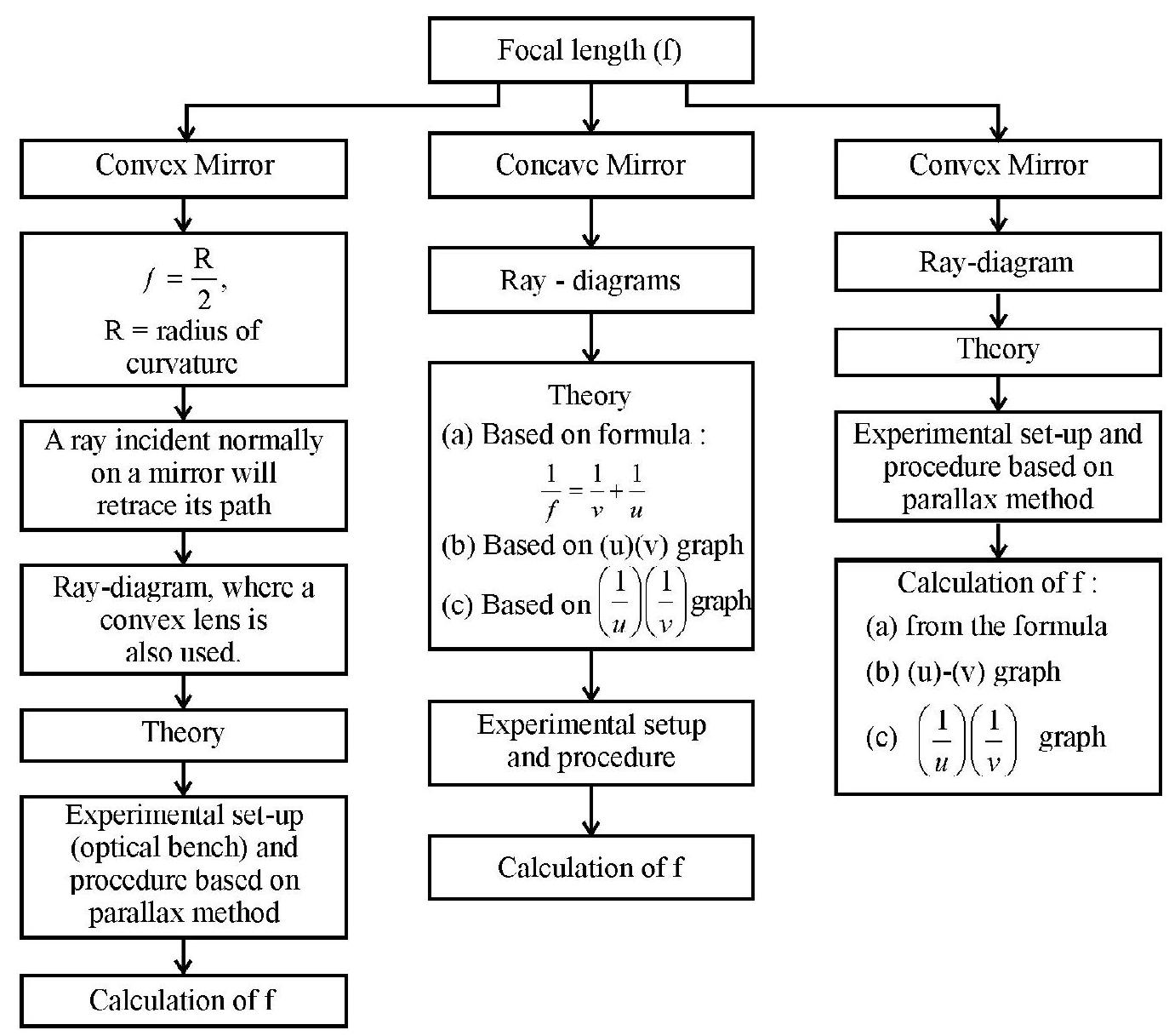
Focal Length (f)
For spherical mirrors (convex and concave mirrors), the focal length (
Now, principal focus, of a spherical mirror, is the point on the principal axis through which (or from which) rays, which are parallel to the principal axis, pass (or appear to diverge from), after reflection from the mirror.

(i) Convex Mirror
A spherical mirror with its reflecting surface convex in shape is alled a convex mirror. The centre of its aperture is named as the pole. The distance of the centre of curvature of the spherical mirror from the pole is called radius of curvature (R). According to the new Cartesian sign conventions, f and R are positive for convex mirror.
(ii)
For small aperture and comparitively longer radius of curvature, the focal length (
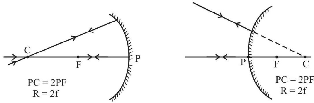
A Ray Incident Normally on a Mirror will Retrace its Path
As per the laws of reflection of light, a ray incident normally on any mirror / surface gets reflected back along the same path.
For a spherical mirror, any ray passing through the centre of curvature (C), or any ray directed towards the centre of curvature, will be incident normally on the mirror. There for they will trace the path back along the incident ray.
Ray-diagram for Detemining the Focal Length of a Convex Mirror, Using a Convex Lens
To determine the focal length (f) os a convex mirror, using the method of parallax, we require a real image to get formed, even while using a convex mirror. For this purpose we use a convex lens, along with the convex mirror. An optical pin is used as the real object here.
Any two rays originating from a point on the pin (for example the tip of the pin, assumed to be on the principle axis of the mirror), will get converged by the lens. If these converging rays are made to get incident normally on the reflecting surface of the convex mirror, they will retrace their path and converge back at the position of the object itself. Thus we will be able to get a real image of the optical pin at the same place where the object itself is.
Conversely, is we obtain a real image of the optical pin at the location of the pin itself, (by adjusting the position of the convex mirror, placed after the convex lens), then we can infer that the rays are incident normally on the surface of the convex mirror.
This scenario is shown in the diagram below.
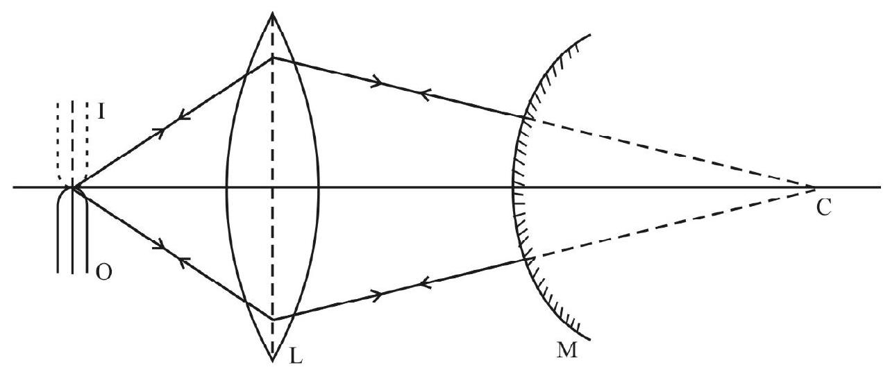
When the mirror is removed, these rays with meet on the right side of the lens, and produce a real image.
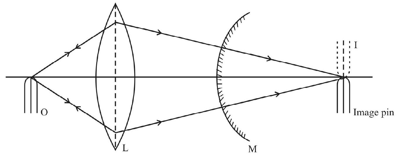
Theory
From the two ray-diagrams drawn, it is clear that the position of the image (I), when the convex mirror is removed will give the centre of curvature of the mirror. (We locate the position of I in the second case by using an image pin and removing the parallax between the image and this image pin).
As image I is formed at ’
Optical Bench
An optical bengh consists of two nickel plated metallic rods of length about
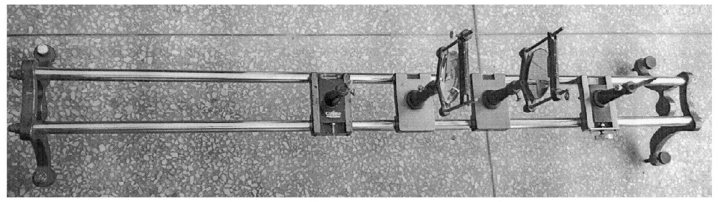
Optical Bench
Parallax Method used to Locate the Position of a Real Image
A real image is formed when two or more rays, originating from a point on the object, are made to actually meet at a point elsewhere, by using optical devices. A real image can be obtained on a screen. In this experiment, the real image, of the optical pin, is located by using the parallax method.
Parallax refers to relative change in position of anobject, with respect to another object, when viewed from different positions. If the relative positions of the objects are different when viewed from different points, we say that there is parallex between such objects. When there is parallax, the objects are at different positions with respect to the viewer.
Now, we can adjust the positions of these objects, with respect to each other, such that the parallax gets removed, or the objects remain at same positions with respect to each other, when viewed from different positions. They may remain coinciding for the viewer, at all positions of the view. This is called removing the parallax. When we remove parallax, between the tips of an image pin and the real image of an object pin, we say that the image (of the object pin) is at the same position as that of the image pin.
To remove parallax in optical experiments we use a refernce optical pin, often called image pin, which is fixed on an upright. When parallax is removed between the real image, and this image pin, the position of the real image is same as that of the image pin and can be noted from the index line of its upright.
Parallax can be removed between the real image of an object pin, and the pin itself also, as is case in the first part of this experiment. While removing the parallex between a real image and the reference pin (image pin), it is advised to observe their relative position using only one eye (keeping the other eye closed).
Procedure for Determining the Focal Length of the Convex Mirror
-
Mount the convex mirror on a holder and then fix the holder on the upright of the optical bench. Simiarly mount a convex lens and fix it on another upright.
-
Place the upright, holding the convex lens, at around
-
Place the convex mirror beyond this lens and at around
-
Now place an object pin
-
Viewing from the same side of the object pin, in the direction of the lens, keeping a minimum distance of
-
Now, remove parallex between this real image and the object pin itself by adjusting the position of the convex mirror. (Ensure that the tip of the image coincides with the tip of the object all the while, during the adjustments we do for the removal of parallax).
-
Once the parallax is removed between the object pin and its image, (formed by the lens and mirror together), we can be sure that the rays, passing through the lens, are falling normally on the convex mirror and so they are getting retraced back, to produce the real image back at the object itself.
-
Record the positions of the object pin, lens and the mirror as
-
Now remove the mirror and place another optic pin, a reference pin (called image pin) on another upright.
-
View the real image, of the object pin, formed by the lens, from the other side of the lens.
-
Make the tips of this real image of the object pin, and the image pin coincide. Adjust the positions of the image pin to remove the parallax, so as to obtain the position of the real image (I) formed by the lens alone.
(Here we are getting the situation corresponding to the second part of the ray-diagram.)
- Record the position of I.
Calculation of
Now, the distance MI will give the radius of curvature of the convex mirror.
Therefore,
But
(To take more observations the position of the object pin can be varied, keeping the position of lens the same. Accordingly the positions of mirror (M) and image (I) will change. But the distance
To find the Focal Length of a Concave Mirror
Concave Mirror
It is a spherical mirror whose reflecting surface is concave in shape. A concave mirror can form real images,on its own, if the object is kept beyond its principal focus (F).
Ray-diagram
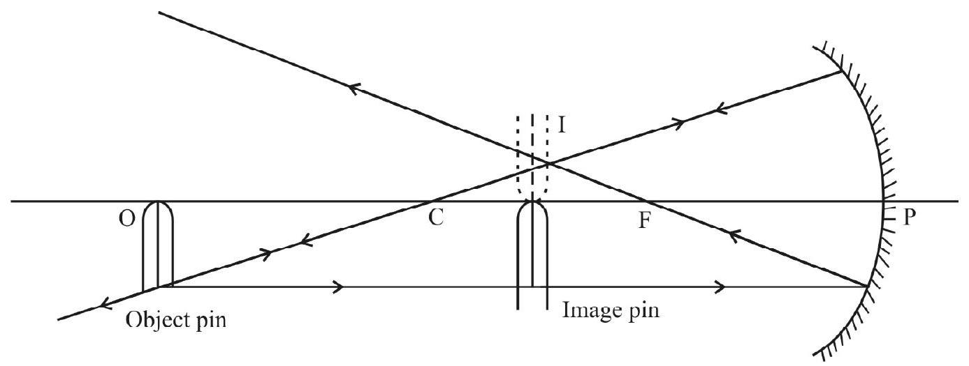
Here, object pin is placed at
Theory
(a) Once we have obtained the values of
Note that both
(b) After we have obtained many values of
After plotting the
But from the geometry,
This means that object and image are at same distance from the pole of the mirror. This happens when they are at
Therefore,
The average of
(c) Corresponding to the various values of
From the graph, it is clear that the co-ordinates of
Therefore
or
Similarly,
The mean of
Experimental Set-up and Procedure
Here also we use the optical bench, with the uprights, as described in case of the convex mirror experiment. The concave mirror is mounted on the upright and this upright is kept at, say,
The object pin is placed at a point which is beyond
Now, using an image pin as reference pin, the parallax, between the image of the object pin and the image pin, is removed to locate the position of the image, accurately. Once the image is located, using the imagepin, the positions of object pin ’
The whole procedure is repeated for different positions of object, each time recording the positions of
In each case:
The focal length (
(a) Formula
(c)
(Note that when
To find the Focal Length of a Convex Lens
Convex Lens
It is a piece of transparent medium bound by two spherical convex surfaces (bi-convex lens).

The centre of the lens is known as optical centre and it is marked as
Focal length (
i.e.
The principal focus
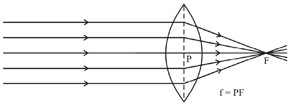
Focal lengh of a convex lens is positive.
Ray-diagram
The convex lens can form real images when the object is kept beyond its
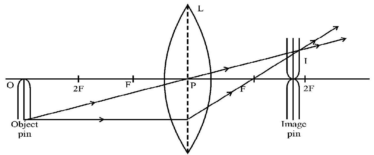
The position of the image (I) is located by removing the parallax between the image pin (reference pin) and the image of the object.
Once the image (I) is located we have
Theory
(a)
(Here
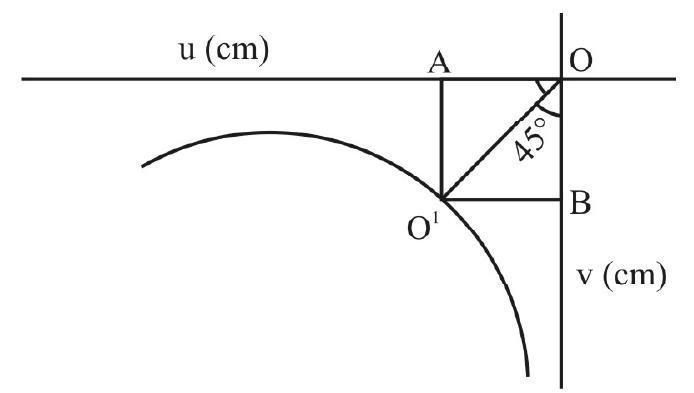
(b) We can plot the u-v graph (in second quadrant) and obtain focal length (f). For plotting (u) vs (v) graph we should use same scale for both ’
Once the graph is drawn, drop the perpendicular and draw the horizontal, as shown.
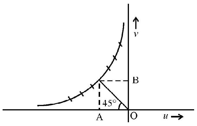
From the geometry if is clear that
Hence
or
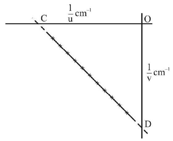
(c) We can also find the values of
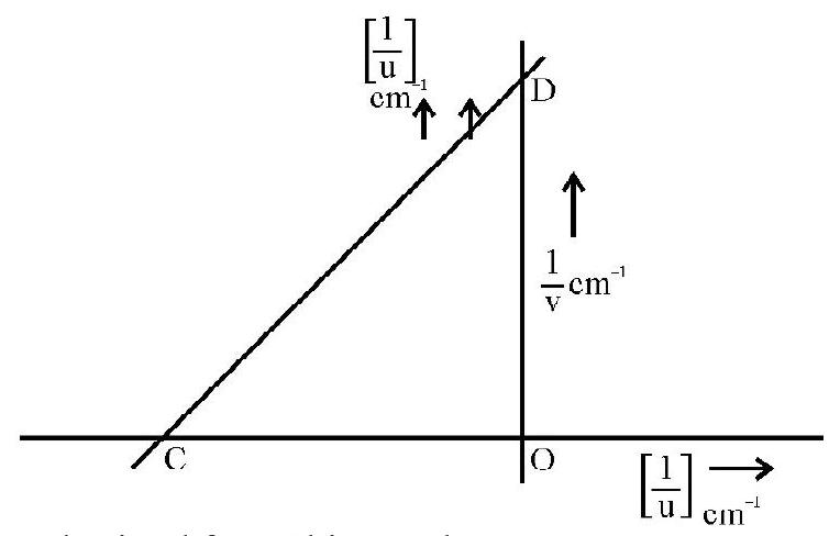
The value of ’
Experimental Set-up and Procedure
The optical bench is used here also. The convex lens is mounted on the upright and it is placed at (around) the
The object pin is placed at a point which is beyond
Now using an image pin, as reference pin, the location of this real image is obtained by removing the parallax between the two.
Once the image is located, the positions of the object pin ’
The procedure is repeated to obtain many values for
Calculations of
(a) From the recorded values of
(b) From the (u) vs (v) graph.
(c) From the
Example:
Astudent, performing the experiment to find the focal length of convex mirror, took the following two sets of observations. Obtain the focal length of the convex mirror.
| Object-pin position (cm) | Lens positions |
Convex Mirror positions when the Image of the object-pin is formed at the object-pin it self |
Image position when the convex Mirror is removed |
|---|---|---|---|
| 70.5 | 50.0 | 42.0 | 31.4 |
| 64.0 | 50.0 | 35.5 | 15.0 |
Show Answer
Solution:
The ray diagram for the first set of observation is shown below.

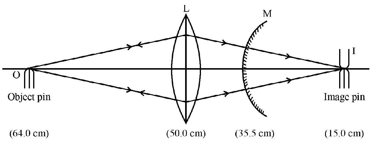
From this, clearly,
From the second set,
Mean
Example:
The following observations were recorded by a student performing concave mirror experiment on optical bench, using parallax method.
| Sr. No. | Position of Mirror |
Position of Object |
Position of Image |
|---|---|---|---|
| 1. | 0.0 | 20.0 | 34.0 |
| 2. | 0.0 | 17.0 | 46.4 |
| 3. | 0.0 | 15.0 | 56.8 |
| 4. | 0.0 | 35.0 | 20.7 |
| 5. | 0.0 | 38.0 | 19.2 |
| 6. | 0.0 | 41.0 | 17.6 |
| 7. | 0.0 | 44.0 | 16.1 |
Calculate the focal length (f) of the concave mirror from these observation by:
(a) calculation using the formula
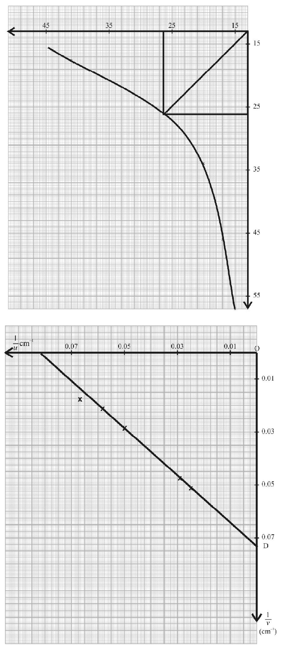
(b) by plotting (u) vs (v) graph.
(c) by plotting
Show Answer
Solution:
In each observation we find the value of
Also we calculate the values of
Finally we calculate
The completed table is shows below:
| Sr. No. | Position of Mirror |
Position of Object |
Position of Image |
|||||
|---|---|---|---|---|---|---|---|---|
| 1. | 0.0 | 20.0 | 34.0 | 20.0 | 34.0 | 0.05 | 0.029 | 12.6 |
| 2. | 0.0 | 17.0 | 46.4 | 17.0 | 46.4 | 0.059 | 0.022 | 12.4 |
| 3. | 0.0 | 15.0 | 56.8 | 15.0 | 56.8 | 0.067 | 0.018 | 11.9 |
| 4. | 0.0 | 35.0 | 20.7 | 35.0 | 20.7 | 0.029 | 0.048 | 14.3 |
| 5. | 0.0 | 38.0 | 19.2 | 38.0 | 19.2 | 0.026 | 0.052 | 12.8 |
| 6. | 0.0 | 41.0 | 17.6 | 41.0 | 17.6 | 0.024 | 0.057 | 12.3 |
| 7. | 0.0 | 44.0 | 16.1 | 44.0 | 16.1 | 0.013 | 0.063 | 11.8 |
(i) Meanf(fromcalculation), using
(ii) (u) vs (v) graph
(iii)
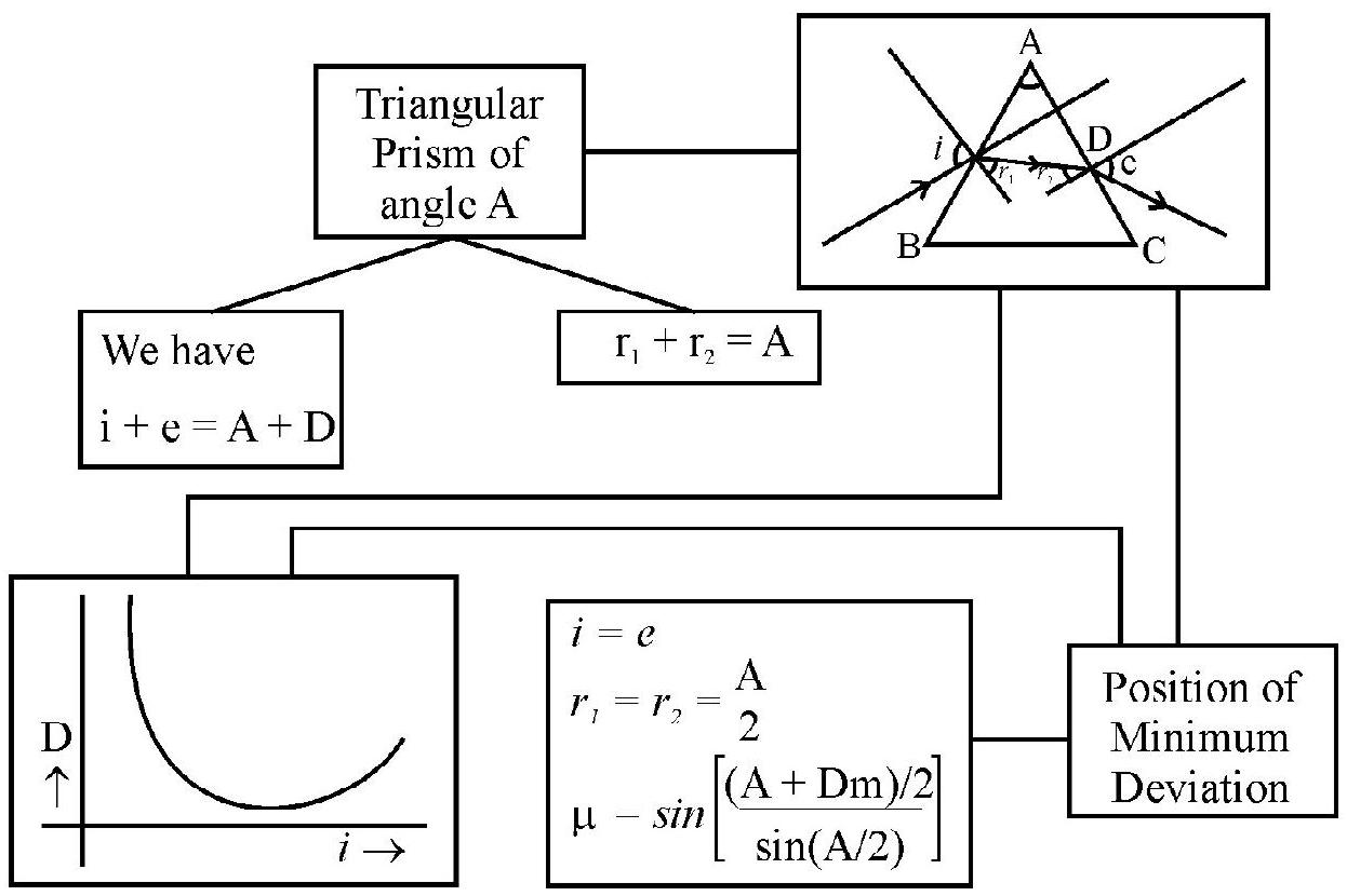
EXPERIMENT–16
Plot of angle of deviation (<D) versus angle of incidence (<i) for a triangular prism.
CONCEPT MAP
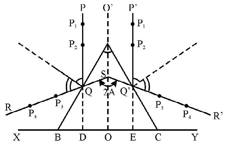
Measurement of the Refracting Angle of the Prism
The refracting angle, of a given prism, can be measured by finding the positions of the reflected rays, corresponding to the incident rays
It can be shown that
Tracing the Path of Rays through a Prism
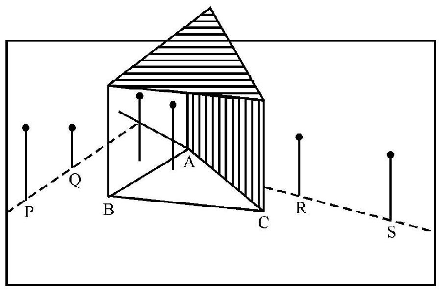
The set up used for tracing the path, of a given incident rays through a prism is as shown. The accompyning diagram shows how the different angles can be measured.
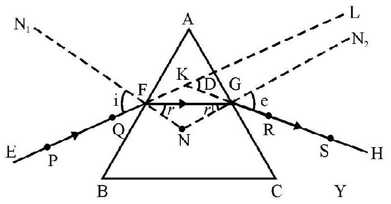
Refraction of Light through a Prism
The ray diagram, showing the refraction of (monochromatic) ray of light by a prism, is given below.
In this diagram
These angles are related as follows:
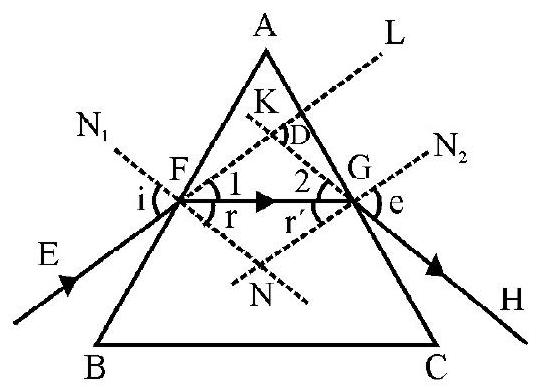
and
Graph between
The dependence of the angle of deviation, on the angle of incidence, is shown in the graph given here.
There is one, and only one, angle of incidence
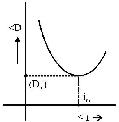
However, there can be two values of the angle of incidence (one greater than
Prism
A prism may be regarded as a section of a transparent medium, bounded by two plane refracting surfaces, meeting at an angle.
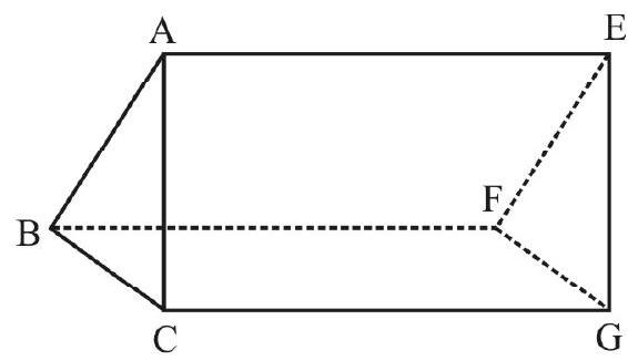
Angle of the Prism
The angle between the two ‘faces’ (surface ABEF and ACGE) is known as the angle of the prism (
Refracting Edge a Prism
The two plane refracting surfaces, of a prism, meet along the line
Principal Section of a Prism
Let a plane, perpendicular to its refracting edge, be used to obtain a ‘section’ of the prism. We refer to such a section as the principal section of the given prism.
Example:
The angle of deviation for a given prism, (made from a material of refractive index
(i)
(ii)
(iii)
(iv)
Solution:
We know that, for a prism,
Here, as D has the same value for the two sets of angles, we have.
EXPERIMENT-17
Refractive index of a glass slab using a travelling microscope.
CONCEPT MAP
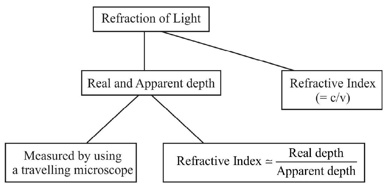
Refraction
There is a change in the speed of light as it goes from one medium to another. The phenomenon, associated with this change in speed of light, are referred to as ‘refraction of light’.
Refraction is usually observed through a change in the direction of propagation (or ‘bending’ of the path) of a ray of light as it goes (obliquely) from one medium to another.
Refractive Index
The refractive index
We also define

Real Depth and Apparent Depth
‘Refraction’ causes a pond of water to appear shallower than it actually is. It can also cause a rectangular glass slab to appear less thick than it actually is.
We use the terms ‘apparent depth’ and ‘real depth’ in this context.
A relation between these two ‘depths’ can be obtained as follows. Consider a rectangular glass slab,
Let there be a point
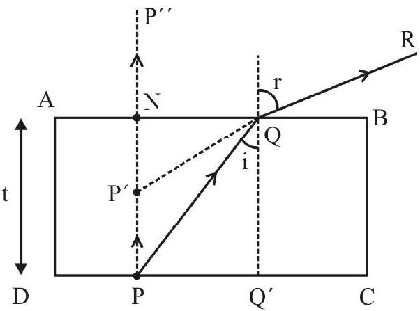
Now, from Snell’s law,
Travelling Microscope
We can use the special microscope, called a travelling microscope, for finding the real and apparent thicknesses of a given glass slab. The ‘stands’, attached to the tube of the ‘compound microscope’ used here, are such that the microscope tube can be moved both ‘up and down’ (i.e. vertically) as well as ‘right and left’ (i.e. horizontally). There are ‘scales’ (‘main scale’, with its attached ‘vernier scale’) that enable one to measure the (vertical or horizontal) movement of the ‘cross-wires’ in the ’eye-piece’ of this microscope. The ’least count’, of the vernier used here is generally

(Travelling Microscope)
To find the apparent depth, of the given glass slab, we put a sharp dark ink mark on a white sheet of paper and focus the microscope on it. Its ‘scale reading’ is taken. The glass slab is now put on top of the mark and the microscope tube is ‘raised up’ so that the image (of the mark) again comes in ‘sharp focus’ of the microscope. The ‘scale reading’ of the microscope is again taken. The difference, between this reading, and the first reading, gives the ‘apparent depth’ of the given glass slab.
To find the ‘real depth’, some lycopodium power, or fine chalk dust, is sprinkled on top of the glass slab. The microscope tube is then raised further till this powder (or dust) particles come in ‘sharp focus’ of the microscope. The scale reading of the microscope is again taken. The difference between this (third) reading, and the first reading, tives the ‘real depth’ of the glass slab.
We then have
Example:
Three different liquids are filled in three beakers to heights
The ratio of their apparent heights, when viewed from above, would be
(i)
(ii)
(iii)
(iv)
Show Answer
Solution:
We have
Apparent depth
or
Example:
A mark, put on a sheet of paper (kept on a table) is viewed from a point at a height
(i)
(ii)
(iii)
(iv)
Show Answer
Solution:
The apparent depth of the glass slab would be
EXPERIMENT-18
Characterstic curves of a pn junction diode in forward bias and reverse bias.
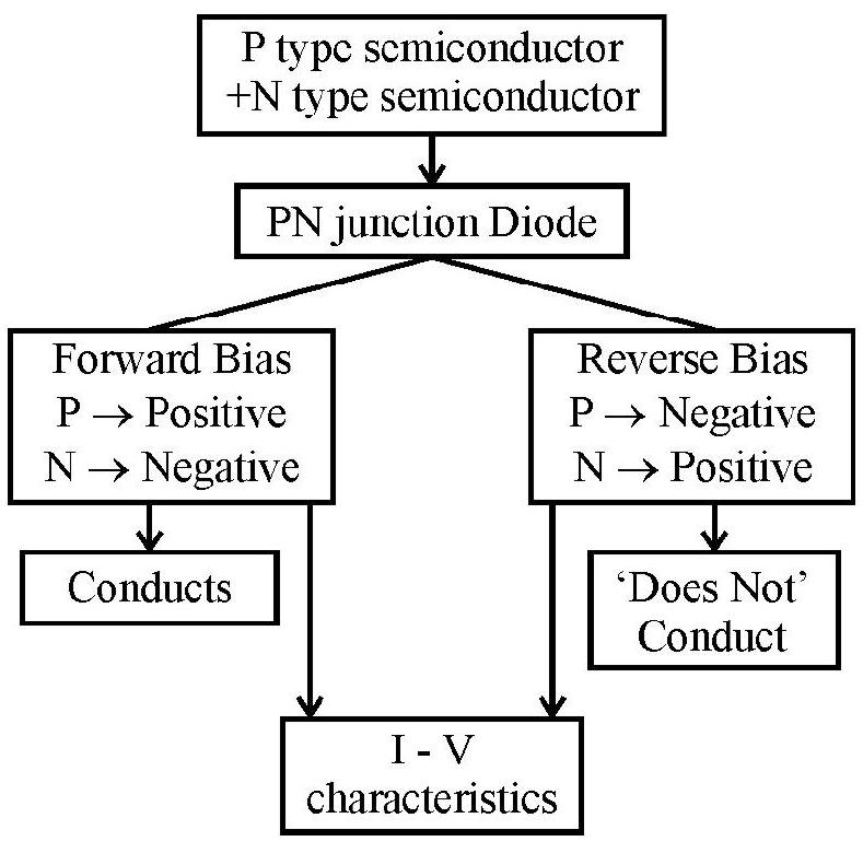
Introduction
A p-n junction is a diode which permits easy flow of currect in only one direction and offers high resistantce to the flow of current in the opposite direction. Fig. (a) shows a p-n junction in forward bias and Fig. (b) shows

The circuit diagram, for studying IV characterstics of a p-n junction diode, is shown below.
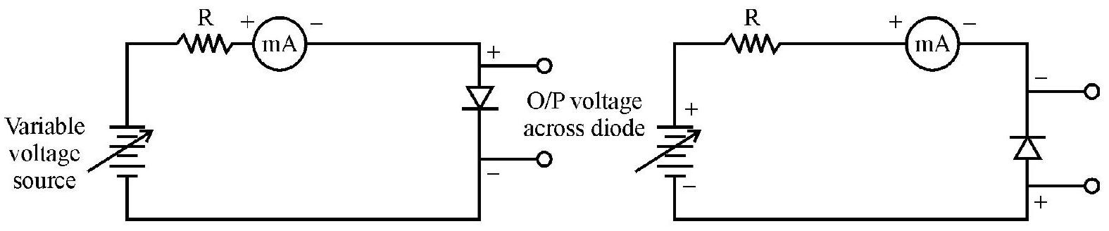
Forward Bias
The external voltage is applied to the diode in such a polarity that the positive terminal is connected to
1. Knee Voltage: It is the voltage across the diode in the forward bias configuration at which the current flowing through the diode starts increasing rapidly.
2. Breakdown Voltage: It is the voltage across the diode, in reverse biased configuration, at which the reverse current suddenly rises; the
3. Avalanche Breakdown: In a normal
The relation between current (I) flowing through the diode (measured by milliammeter), the voltage drop (V) across the diode (measured by connecting either a voltmeter or a multimeter), is given by.
Here, Is
Therefore, in forward bias,
1. When external voltage is zero, then no current flows through the diode.
2. As voltage increases, potential barrier of the
In this region,
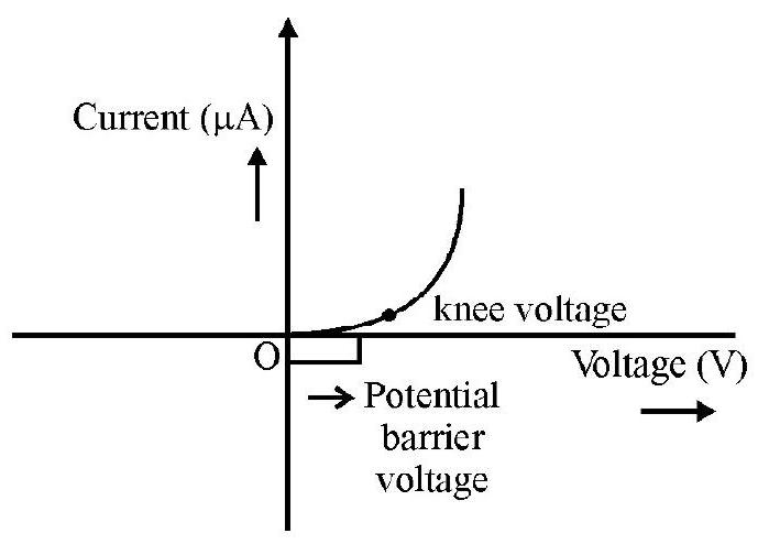
Reverse Bias
The external voltage is applied to the diode such that, the positive terminal of the voltage is connected to ntype end of the diode and negative terminal is connected to
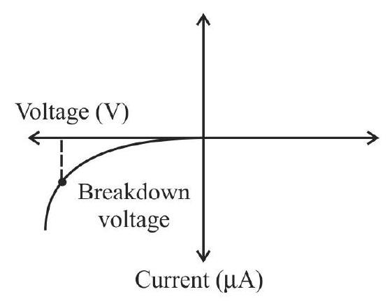
If reverse voltage is increased, the kinetic energy of minority carriers increases; they may then remove electrons from the semiconductor atoms. This stage is called as breakdown of the junction; the voltage, at which it occurs, is called as the breakdown voltage.
EXPERIMENT-19
Characterstics curves of a Zener Diode and finding the Reverse Breakdown Voltage.
CONCEPT MAP

Introduction
Zener diode is a diode having heavily doped
The I-V characterstics curve of a Zener diode in forward bias configuration is similar to that of a
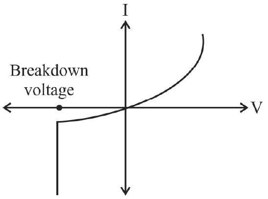
The breakdown voltage is sometimes called as Zener voltage; the corresponding current is called as ‘knee current’.
The breakdown voltage depends on the extent of doping. It doping is high, the depletion layer is very thin; as a result, the breakdown occurs even at a lower reverse voltage.
In order to determine the reverse breakdown voltage of a zener diode the following circuit is made.
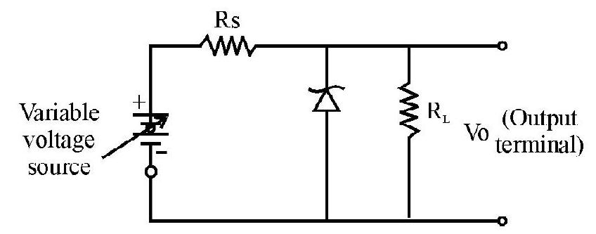
The input voltage
When
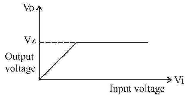
EXPERIMENT–20
Characterstic curves of a transistor and finding current gain and voltage gain.
CONCEPT MAP
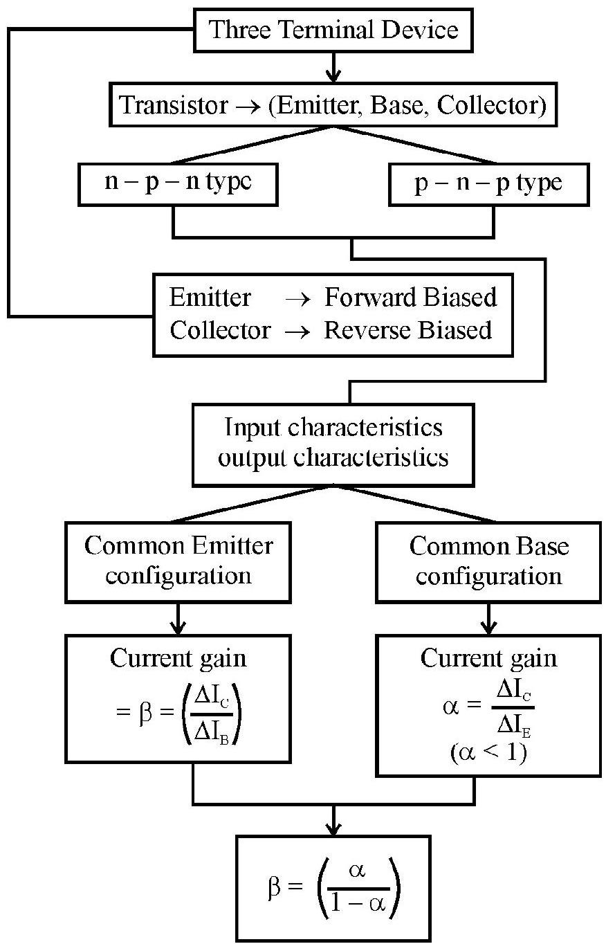
Introduction
We known that the transistor is a three terminal device that is used for a wide variety of practical applications.
The simple junction transistor has two well known forms: the
A pnp transistor is normally biased in the manner shown here.
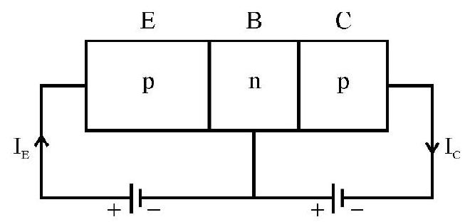
For a n p n transistor, all the polarities will change.
In normal transistor action, the emitter-base junction is forward biased and collector-base junction is reverse biased. Due to forward bias, the holes in the p-type emitter flow towards the n-types base. This flow of holes constitutes the emitter current
Therefore,
Some “Facts” about the Transistor
1. A transistor has 3 regions - emitter, base and collector. The base is the thinnest and is only lightly doped. Due to this, it passes most of the charge carriers from emitter to collector.
2. Emitter is heavily doped becuase it has to inject charge carriers into the base.
3. Collector region is the largest and is moderately doped.
Circuit diagram for
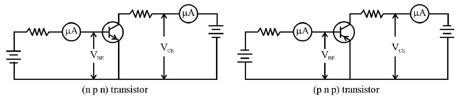
Input Characterstics
It is a curve between base curcuit
1. It resembles the IV characterstics curve of a forward biased diode. It is so because the emitter-base junction is forward biased and acts like a diode.
2. Initially base current is very small. It increases sharply once the input voltage ( or
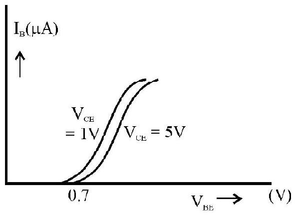
3. If the (reverse) collector voltage is increased, then, for the same
Output Characterstics
It is a curve between base curcuit
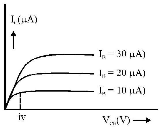
It should be noticed:
1. Initially collector current increases with base current. But after about
The small slope, in the IV curve, beyond knee voltage is because of the collector depletion layer which gets wide enough (due to reverse collector setting), to capture majority charge carriers.
2. Current gain: It is ratio of change in collector current to the change in base current.
Generally value of
In common base configuration, current gain is defined as
Value of
3. Relation between
EXPERIMENT-21
Identification of diode, LED, transistor, IC, resistor, capacitor from a rised collection of such items.
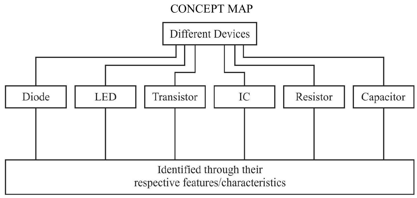
Introduction
We know that the diode, LED, transistor, IC, resistors and capactiors are widely used in different electronic and electric circuits. It is important, therefore, to get familiar with their basic characterstics and the simple ways to identify them, from a mixed collection of such items.
We now talk about each of these devices in some detail.
1. Resistor
(i) A resistor is a small electric/electronic device that resists the flow of electric current. It obeys Ohm’s law which states that the current I flowing through a resistor (having resistance
I
(ii) The commanly used resistor in practical laboratories are the (two terminal) colour coded carbon resistors. They generally have four colours stips. The first three colour signify the the value of resistor the fourth colour implies the tolerance rating. The colour and their respective numbering is as follows:
Golden
Silver
B Black 0
B Brown 1
R Red 2
| Orange | 3 | |
|---|---|---|
| Y | Yellow | 4 |
| G | Green | 5 |
| B | Blue | 6 |
| V | Violet | 7 |
| G | Grey | 8 |
| W | White | 9 |

If the four folour are: yellow, red, red golden, it implies that the resistance
(iii) Resistor is a passive device its the two terminals are not categorized as cathode / anode or as
(iv) Place the multimeter knob on the dial marked will the symbol ’
2. Diode and LED
(i) Diode and LED are semiconductor devices which consist of two semi conductor layers forming a p-n junction. LED (light emitting diode) is a special type of diode which has the capacity of emitting light.
(ii) The diode and the LED, both have two terminals and one of them is the (p-type) positive anode terminal. The other is the (n-type) negative cathode terminal.
The lengths of wires, joined to the positive and negative terminal, are different.
LED
(a)
-
The longer leg is the
-
The shorter leg is the (
[Note: This is not the best identification criteria because some manufacturers offer the polarity in the reverse way also].
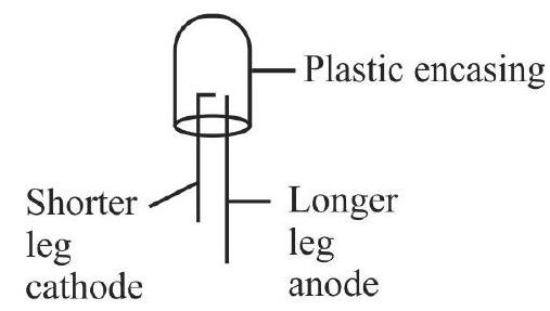
(b) If the lengths of the two terminals is same, then look inside the plastic casing. The flat-flag type end correponds to the cathode (
(c) There are no coloured striped markings in the LED.
(d) Generally, there are no number codes on an LED.
(e) Connect positive probe of the multimeter to the anode of LED and also place the negative (common) probe of multimeter on the cathode of LED.
Put the knob of the multimeter on the ‘diode’ symbol. You will see that LED will light up in this forward bias configuration. The display will show a value
Diode
The anode and cathode of diode can be identified through the marking of a strip. Towards one end of the diode, a shaded band type marking is made. The signifies the cathode of the diode. Generally, normal diodes are black coloured with a grey-silver band type strip. [Remember: In a resistor, we have four coloured strips, but in a diode, we have only one strip!!]. Diode have low resistance to flow of current in one direction and a very high resistance in the other direction.
The diodes are always numbered. The numbering code, however, varies from one manufacturer to another. For example in American system, the code is like IN4007 which implies that it is a normal, diode, having tolerance of
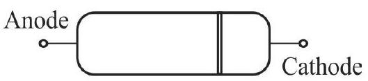
By using multimeter, the diode can be identified as follows:
Connect multimeter probes to the diode terminals as per its forward biased configuration. Put the multimeter knob on ‘diode’ symbol. The display will show
3. Capacitor
Capacitor is also a two terminal device, but (as compared to resistance and diode) it is generally not colour coded. Most capacitor have capacitance value written on them.
(a) This is typical example of non-electrolytic (casing) capacitor. There is no anode / cathode
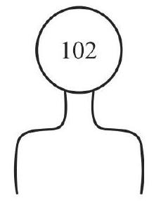
(b)
- Electrolytic cylindrical aluminimum casing.
4.7
-
The two terminals are of different lengths.
-
Longer leg is +ve (anode).
-
Shorter leg is-ve (cathode).
-
Sometimes ‘-’ minus sign is also drawn on the cap.

4. Transistor
Transistor is a three terminal device; it can be easily identified from a collection of items (
5. IC
Integrated circuit (IC) is one in which components such as diodes, transistors, capacitors and resistors etc. are embeded on a small semiconductor chip. The size of IC is so small that one will require a microscope to see the connection between these components. The ICs are protected from external disturbances by encapsulating them in plastic / metal/ ceramic packages. We generally have the IC package shown here.
It is a flat pack container having equal number of pins on either side. The total number of pins can be
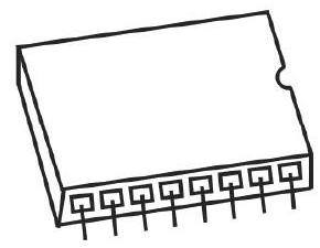
Example:
The colour coding of a resistor is brown, black, red, golden.
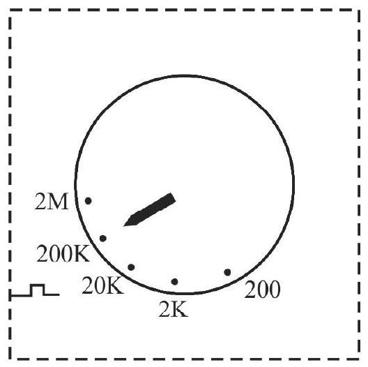
(i) What will be the most likely value displayed when the multimeter knob is at ’
(a) 1.003
(b) 1.00
(c) 01.0
(d) 0.001
(ii) What will be the most likely value displayed when knob is at ’
(a) 1.003
(b) 1.00
(c) 01.0
(d) 0.001
(iii) What will be the most likely value displayed when knob is at ’
(a) 1.003
(b) 1.00
(c) 01.0
(d) 0.001
(iv) What will be the most likely value displayed when knob is at ’
(a) 1.003
(b) 1.00
(c) 01.0
(d) 0.001
Solution:
(i) (a)
(ii) (b)
(iii) c
(iv) (d)
Reason: Brown black red
Golden
Value of resistor lies between
For best precision, knob should be placed at the next higher position i.e.
where
Precision in measurement decreases if the knob is placed at other higher markings.
EXPERIMENT-22
Use multimeter to identify: base of a transistor; distinguish between npn and pnp transistor; see unidirectional flow of current in case of a diode and a LED.
CONCEPT MAP
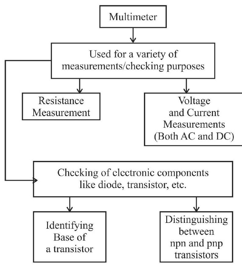
Introduction
We know that the multimeter is an integral and essential part of an electronics or physics laboratory. It is put to many uses. Here we will try to understand its uses with respet to a transistor and a diode.
The basic details of the use of a multimeter for doing the indicated identifications, in case of a transistor and a diode/LED, are outlined below. We first do a brief recapitulation of the basic features of a multimeter.
The Multimeter
Multimeter basically has 3 important parts:
(a) Display Section: Here generally 4 digits value, and +/sign of the quantity being measured, is displayed.
(b) Selection Knobs: It allows the user to set the multimeter to read different quantities such as current (ac/dc), voltage (ac/dc), resistance, capacitance etc.
(c) Two probes which are inserted in the ports present at the bottom. One of the probe is connected to COM (ground) port; the other is connected to either of the ports depending on the quantity to be measured.
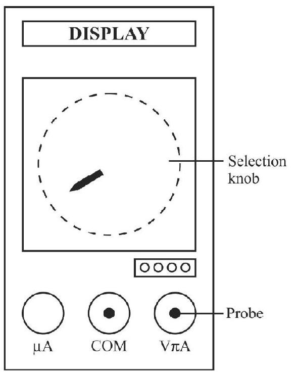
Identification of Base of Transistor
Physically
(i) In some transistors, there is a notch. The leg / pin, next / nearest to the notch, is emitter. Moving ahead in clockwise direction (pins towards the user) gives base and the collector.
(ii) Some transistors have a black flat top which is rounded on one end. Keep flat surface towards you and the pins pointing upwards. Emitter, Base and collector will be as shown in the diagram.

Using a Multimeter
(i) Transistor are either
Put -ve probe of multimeter to one of the pins. Put selection knob on the ‘diode’ symbol. Put +ve probe to other 2 pins. A value
Only in
Whenever -ve probe is at pin *, then
Distinguish between npn and pnp Transistor
In the previous article, we identified the base of transistor. Once base is identified, the type of transistor,
There is one more method.
Put knob on ’ 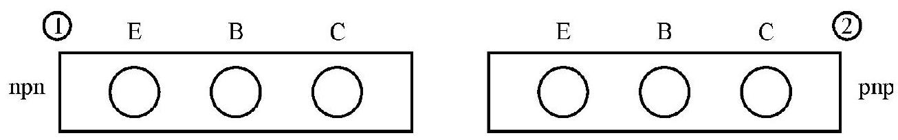
Put E,B, C of transistor in (1). If it is npn transistor, then it will show
Unidirectional Flow of Current through Diode / LED
We have seen in previous experiment, that when knob of multimeter is placed on ‘diode’ symbol, then diode shows
PROBLEMS FOR PRACTICE
1. The main scale, of a given vernier scale set up, has been gradiented to read up to
The zero error of this vernier equals (-2) times its least count. The readings, in a given case, are as follows:
Main scale reading
The corrected value of this reading is
(1)
(2)
(3)
(4)
Show Answer
Answer: (1)2. In a given vernier callipers,
(i) Main scale reads (m) units
(ii) The
(1)
(2)
(3)
(4)
Show Answer
Answer: (2)3. A given screw gauge has a least count of
When this scrw gauge, is used to measure the thickness of a thin mica sheet, the main scale reads 0.7
The ‘pitch’ of this screw gauge, and the thickness of the mica sheet, are respectively, equal to
(1)
(2)
(3)
(4)
Show Answer
Answer: (3)4. The pitch, of a given screw guage, equals (p)
When a thin wire is just held between the jaws of the screw guage, the main scale reads
(1)
(2)
(3)
(4)
Show Answer
Answer: (1)5. The energy, of the bob of a simple pendulum, decreases to
(1)
(2)
(3)
(4)
Show Answer
Answer: (1)6. The graph showing the variation, of the square of the amplitude
(1)
(2)
(3)
(4)
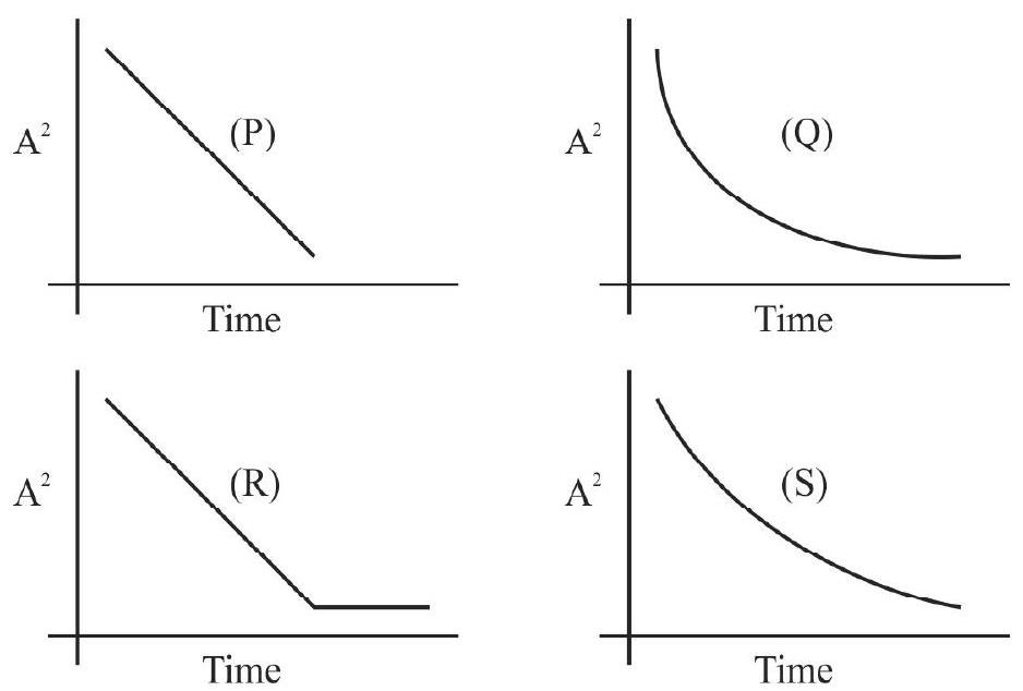
Show Answer
Answer: (2)7. The meter scale gets balanced in the set-up shown here. The mass,
(1)
(2)
(3)
(4)
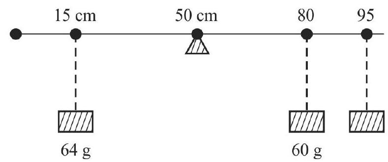
Show Answer
Answer: (4)8. The mass of the meter scale that gets balanced, in the set-up shown, equals (nearly)
(1)
(2)
(3)
(4)
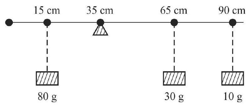
Show Answer
Answer: (4)9. Two wires, made of materials
(1)
(2)
(3)
(4)
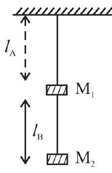
Show Answer
Answer: (1)10. N idential hollow cylindrical columns, made from a metal of Young’s modulus
(1)
(2)
(3)
(4)
Show Answer
Answer: (4)11. Water, (assumed to ‘spread out’ on glass), rises to a height
If the same capillary tube were to be dipped in mercury (surface tension
(1) at a height h’ where h’
(2) at a depth
(3) at a depth
(4) at a height h" where
Show Answer
Answer: (3)12. The difference, in the mean value of the readings of the travelling microscope, when its horizontal ‘cross wire’, is at the two positions, indicated here, equals
This capillary tube is dipped in a liquid of surface tension
the liquid with the walls of the capillary tube, is
(1)
(2)
(3)
(4)
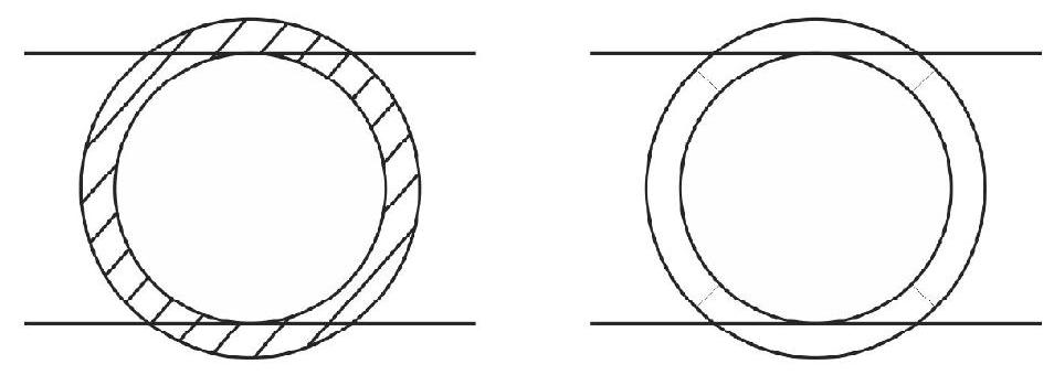
Show Answer
Answer: (2)13. An oil drop (density of oil
(1)
(2)
(3)
(4)
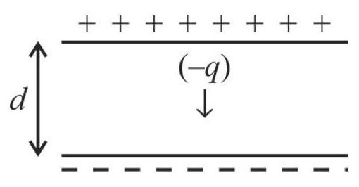
Show Answer
Answer: (3)14. Adrop of a liquid (of density
Another drop of another liquid (of density
(1)
(2)
(3)
(4)
Show Answer
Answer: (4)15. The (temperature) vs (time) graph, of a body (initially at a temperature
(1)
(2)
(3)
(4)
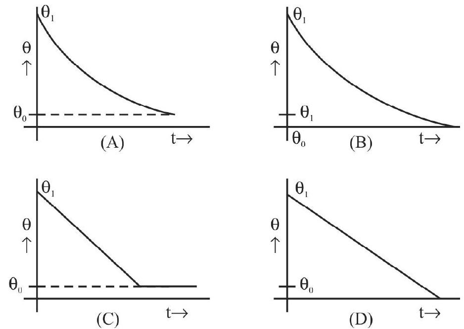
Show Answer
Answer: (1)16. Ahot body, initially at a temperature
(i)
(ii)
We can then say that
(1)
(2)
(3)
(4)
Show Answer
Answer: (3)17. A student does the experiment on finding the speed of sound using a resonance tube. He uses a resonance tube of diameter
(1)
(2)
(3)
(4)
Show Answer
Answer: (2)18. The speed of sound in air, at
(1)
(2)
(3)
(4)
Show Answer
Answer: (1)19. A given solid, of mass
(1)
(2)
(3)
(4)
Show Answer
Answer: (1)20. The quantity of heat needed to bring a rise
(i) mass
(ii) mass
If the quantity of heat needed to bring the same rise
(1) zero
(2)
(3)
(4)
Show Answer
Answer: (3)21. An equilateral prism is made from a material of refractive index
(1)
(2)
(3)
(4)
Show Answer
Answer: (4)22. A ray of light, incident on one face of an equilateral prism (made from a material of refractive index
(1)
(2)
(3)
(4)
Show Answer
Answer: (1)23. The forward and reverse currents, flowing through a diode, are due respectively to
(1) Majority charge carriers for both the currents.
(2) Minority charge carriers for both the currents.
(3) Majority charge carriers and minority charge carriers.
(4) Minority charge carriers and majority charge carriers.
Show Answer
Answer: (3)24. The knee voltage, for Ge and Si diode are (respectively)
(1)
(2)
(3)
(4)
Show Answer
Answer: (2)25. Zener diode, having a Zener voltage
(1)
(2)
(3)
(4)
Show Answer
Answer: (4)26. A zener diode is generally used as,
(1) p-n junction diode
(2) Full wave rectifier
(3) Half wave rectifier
(4) Voltage regulator
Show Answer
Answer: (4)27. A characterstics feature of IV graph of a Zener diode is
(1) Gradual reverse breakdown
(2) Gradual forward breakdown
(3) Sudden reverse breakdown
(4) Sudden forward breakdown
Show Answer
Answer: (3)28. In a CE transistor (in active mode), the emitter-base junction has a resistance (
(1) low resistance, low resistance
(2) high resistance, high resistance
(3) low resistance, high resistance
(4) high resistance, low resistance
Show Answer
Answer: (3)29. The input characterstics curves of a transistor, are curves between
(1) Input current and output voltage for fixed input voltage.
(2) Input current and input voltage for fixed output voltage.
(3) Output current and output voltage for fixed input voltage.
(4) Output current and input voltage for fixed output voltage.
Show Answer
Answer: (2)30. Two multimeters (A and B) require a total markings of
(1) A will measure
(2) B will measure
(3) A and
(4) B has a better ’least count’ than A.
Show Answer
Answer: (1)Question Bank
Key Learning Points
Experiment-1: Vernier Callipers
1. The vernier callipers has a vernier scale that slides on its main scale.
2. The least count of a vernier equals the difference between the values of its 1 main scale division and 1 vernier scale division. It is usually calculated by using the ‘formula’
3. The read a vernier, we read / observe
(i) the main scale reading
(ii) the number (n) of the vernier scale division the coincides with some division on the main scale.
The complete reading is then
4. A vernier callipers is said to have a ‘zero error’ if the zeroes, of its main scale and its vernier scale, do not coincide when the jaws of the vernier just touch each other.
5. The zero error is positive / negative if the zero of the vernier scale lies to the right / left of the zero of the main scale. (when the jaws of the vernier just touch other).
6. The ‘zero error’ is always subtracted algebraically, from the observed reading, to get the corrected reading.
Experiment-2: Screw Gauge
7. Ascrew gauge has an accurately threaded screw, having a closely fitting nut whose threadings match that of the screw.
8. The screw, when rotated, has a simultaneous rotatory motion along a circular path and a translatory motion along a straight path.
9. The linear distance, moved by the screw in one complete rotation, is known as its ‘pitch’.
10. The least count, of a screw gauge, is obtained by dividing its pitch, by the number of divisions on its circular scale.
11. To read a screw gauge, the ‘object’/dimension,to be measured, is just held between the jaws of the screw gauge. One then notes its main scale reading (say ’
12. The screw gauge is said to have a ‘zero error’ if the zero of its circular scale, lies above / below the ‘reference line’, when the jaws of the screw gauge are just in contact with each other.
13. The magnitude of the ‘zero error’ is obtained by multiplying the ’least count’ with the number of divisons of the circular scale, by which its zero is above / below the reference line.
14. The ‘zero error’ is negative if the ‘zero’, of the circular scale (when the jaws of the screw gauge are just in contact with each other) lies above the ‘reference line’. It is positive if this lies below the reference line.
15. The ‘zero error’ is always subtracted algebraically from the observed readings.
16. A screw gauge, that has been in use for long (or has a manufacturing defect), can develop some ‘play’ in the motion of its screw. The screw then may not advance even when it is being rotated. This error is known as ‘backlash error’.
17. The ‘backlash error’ can be avoided by rotating the screw in one direction only.
Experiment-3: Simple Pendulum
18. A simple pendulum is made by attaching a small heavy spherical metal bob to a good quality sewing (cotton) thread.
19. The oscillations of a simple pendulum are simple harmonic only if the amplitude of its oscillations is small.
20. The oscillating bob, of a simple pendulum, has both kinetic as well as potential energies.
21. The total energy of the oscillating bob of the pendulum, equals
22. When the bob is oscillating in a medium (like air), its oscillations are damped (harmonic) oscillations.
23. The amplitude of (damped) oscillations decays exponentially with time.
24. One can observe the variation of amplitude with time, and use it to draw a graph between the square of amplitude (a measure of the energy) of the oscillating bob, with time.
25. The above graph is expected to be an exponentially decaying curve.
Experiment-4: Principle of Moments
26. We define the magnitude of the moment of a force, about a given point (or axis), as the product of the force and the ‘force-arm’. Here the ‘force-arm’ equals the perpendicular distance between the line of action of the force and the axis (or point) about which rotation is taking place.
27. The vector relation giving the magnitude as well as the direction of the moment
Here
28. The principle of moments says that
“Whenever a body is in equilibrium under the action of a number of coplaner forces, the algebraic sum of the moments of all there forces, about any arbitrary point, is zero.
29. We take anticlockwise moments as +ve and clockwise moments as (-)ve.
30. We can use the principle of moments to find an unknown mass, by using a meter scale and a known mass.
31. We can also use the principle of moments to find the mass of the meter scale itself.
Experiment-5: Young’s Modulus
32. “The tendency, to regain the original conditions, after the removal of the deforming forces”. This characterstics of materials is known as elasticity.
33. The stress developed, in a deformed object, equals the internal restoring force, measured per unit area.
34. Strain equals the ‘change in dimension’ per unit dimension.
35. According to Hook’s law:
“For smalls values of strain the stress, developed in an object, is proportional to the strain produced in it”.
36. Within the elastic limit:
37.
38.
39.
40. The Si unit, of all moduli of elasticity, equals
41.
42. Searle’s appraratus is used for experimental measurement of Young’s modulus of the material of a wire.
Experiment-6: Surface Tension
43. The forces, which the atoms / molecules of a material exert on one another, are known as interatomic / intermolecules forces.
44. Interatomic / intermolecular forces are short ranged altractive forces; however, these forces become repulsive in nature if the atoms / molecules come too close to each other.
45. Interatomic / intermolecular forces are known as cohesive forces if they exist between similar atoms / molecules. For different types of atoms / molecules, these forces are known as adhesive forces.
46. The property of a liquid surface, to be in a state of stress, is referred to as the phenomenon of surface tension.
47. The surface tension of a liquid is measured in unit of
48. The shape of the meniscus of a liquid, when put in a container, is used to define a term called the ‘angle of contact’.
49. The addtional potential energy, of the molecules of a liquid on the surface of the liquid, is referred to as their surface energy.
50. The surface energy per unit area of the liquid surface, equals the surface tension of the liquid.
51. There exists an ’excess of pressure’ on the concave side of the curved surface of a liquid.
52. The excess pressure, on the concave side of the curved surface
(i) equals (
(ii) equals (
Here
53. The level of a liquid, in a capillary tube dipped in a container of the liquid, is different from the general level outside the capillary tube.
54. The difference in levels (h), inside the capillary tube and the container outside, is related to the surface tension
Here
55. We generally use a specially designed ’travelling microscope’ for finding the surface tension of a liquid by the capillary rise method.
Experiment-7: Viscosity
56. Viscosity may be viewed as a sort of ‘internal friction’, between adjacent liquid layers having a ‘relative motion’ between them.
57. According to Newton’s law of viscous flow:
(
58. The Si and CGS units of
59. According to Stokes’ law
60. The ’terminal velocity’, of a falling ball, is that value of its velocity at which the viscous force, on it, just equals its net downward ‘weight’.
61. The formula, for terminal velocity, is
62. The slope (
Experiment-8: Temperature - Time Graph
63. The basic heat transfer formula: Heat gained = Heat lost
64. The transfer of heat takes place through the processes of conduction, convection and radiation.
65. Conduction is important in case of solids; convection is generally the main method of heat transfer in fluids; ‘radiation’ can cause heat transfer even in vacuum.
66. A hot body, kept in ‘isolation’, losses heat mainly through the processes of convection and radiation.
67. The heat energy, emitted through radiation, is quantified through Stefan’s law.
68. According to Stefan’s law:
“The heat radiation, emitted per unit area per second by a perfectly black body, is directly proportional to the fourth power of its absolute (kelvin) temperature”.
69. When the (kelvin) temperature of a perfectly black body is close to the (kelvin) temperature of its surroundings, the net heat radiated by it per unit area per second, is (approximately) directly proportional to the excess of its temperature over the surroundings.
70. According to Newton’s law of cooling:
“The rate of fall in temperature, of a hot body, is directly proportional to the difference in temperature between the hot body and its surroundings”.
Thus,
71. Newton’s law of cooling leads to the result:
Thus the graph between
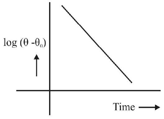
72. It is not quite correct to regard Newton’s law of cooling as an approximation of Stefan’s law.
73. Newtono’s law of cooling is relevant to cooling by convection. When cooling takes place primarily through convection, Newton’s law is (quite) valid even for relatively large difference of temperature between the hot body and its surroundings.
Experiment-9: Resonance Tube
74. Stationary waves are formed through the superposition of a direct wave with its own reflected wave, propagating in the opposite direction.
75. We can get stationary form waves formed in an air column, contained in an open or a closed tube.
76. The permissible modes of vibration of the air column, in an open tube, can have frequencies that are all integral multiples of its fundamental (or simplest) frequency.
77. The permissible modes of vibration, of the air column, in a closed tube, can only have frequencies that are odd integral multiples of its fundamental or simplest frequency.
78. A tuning fork produces a note of a single (constant) frequency that is characterstic of the given tuning fork.
79. The phenomenon of resonance takes place when the frequency of the applied periodic force (used to vibrate a given system) matches the natural frequency of the system itself.
80. The phenomenon of resonance is used in a ‘resonance column set up’ to find the speed of sound in air.
81. The ’end-correction’, associated with the (resonance column) set up, can be eliminated by observing the first and second positions of resonance.
82. The formula used is:
Experiment-10: Specific Heat Capacity
83. The ‘quantity of heat’ is calculated by using the formula
84. We define the ‘specific heat capacity’, of a substance, as the quantity of heat needed to bring a unit change in the temperature of a unit mass of the substance.
85. The thermal capacity of a substance is the product of its mass and the specific heat capacity of its material.
86. We use the ‘calorimeter’ for doing simple heat related experiments in the laboratory.
87. In the ‘method of mixtures’, the hot body is made to transfer its heat to the cold body that is usually contained in a calorimeter.
88. We can use the formula
for finding the specific heat capacity of a solid. Here (
89. We have a similar formula for finding the (unknown) specific heat capacity of a liquid.
Experiment-11: Meter Bridge
90. Wheatstone’s bridge is an arrangment consisting of five resistances
91. When the Wheatstone’s bridge is balanced, by adjusting the known variable resistances
92. Wheatstone’s bridge is used to find the value of an unknown resistance (s), usually connected in the fourth arm, from the Wheatstone’s condition for balacing:
93. Metre bridge is a modified form of Wheatstone’s bridge.
94. Metre bridge is convenient for doing experiments on finding an unknown resistance.
95. The name ‘Metre bridge’ is derived from the fact that it consists of a one ‘metre’ long uniform resistance wire, fixed on a wooden board.
96. Metre bridge is also called slide-wire bridge.
97. The value of the unknown resistance
where
98. Specific resistance, or resistivity (
99. Specific resistance, of the material of a given wire, of length
100. For metre bridge, the value of
101. The thick metal strips, used in the metre bridge apparatus, provide negligible resistance (almost zero) between verious terminals.
102. Loose contacts, at the terminals, or the plug-keys, will cause error in the determination of X.
Experiment-12: Ohm’s Law
103. Ohm’s law states that current flowing through a conductor is proportional to the potential difference across its ends, when the physical conditions are kept constant.
104.
105.
106. Resistance can be viewed as the obstruction offered by the conductor against flow of charges.
107. Resistance is caused due to collisions between moving charges and atoms / molecules of the conductor.
108. Resistance depends on
(a) the nature of the material.
(b) the length of the conductor/wire.
(c) the area of cross-section of the wire.
(d) the temperature of the wire.
109.
(
110. The relation:
111.
112. When the temperature coefficient of resistance is negligible
113. If the resistance of a wire is constant, the graph plotted, for different values of
114. If
115. If
116. The slope of
Experiment-13: Potentiometer
117. Electrochemical cells, called simply as cells, convert chemical energy into electrical energy.
118. Daniel cell and Leclanche cell are primary cells which can’t be recharged.
119. Lead-acid accumulator, or acid battery, is a secondary cell; it can be recharged.
120. Every cell has got an EMF which is measured not as a force but in terms of work done per unit charge.
121. There are two definitions of EMF of a cell:
(i) In terms of work done: “EMF of a cell is defined as the work done in driving one coulomb of charge through a (closed) circuit, including the cell
(ii) In terms of terminal voltage
122. Internal resistance (
123. Internal resistance (
124. Terminal voltage
(Terminal voltage is the potential difference across the external circuit).
125. The terminal voltage
(i)
or (ii)
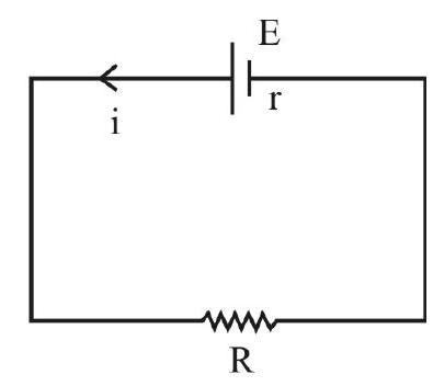
126. The principle of potentiometer is that when a steady current (I) is maintained in the uniform wire of the potentiometer, the potential difference
i.e.
or
127.
128. Lower is the value of potential gradient, greater will be the accuracy of measurements.
129. The formula used for comparison of EMFs, using potentiometer, is
130. The formula used for determining the internal resistance of a primary cell is:
Experiment-14: Moving Coil Galvanometer
131. Galvanometer is an extremely sensitive device, used to detect even very small currents.
132. A galvanometer works on the principle. “A current carrying coil, when suspended in a magnetic field, experiences a torque”.
133. Normally a galvanometer is provided with a linear scale with zero at the centre and with 30 equal divisions on either side of the zero. A pointer, attached to the coil, can deflect and move over the scale, whenever the current passed rotates the coil of the galvanometer.
134. The resistance (G) of the galvanometer is the resistance of the (copper) coil in it. It may (usually) be between
135. Figure of merit, (k), is the current required to produce one division deflection in the galvanometer. It is given by
where
136. The unit of k is ampere-divisions
137. The formula for finding G, by the ‘half deflection method’, is
Here
138. The formula for finding
Here
Experiment-15: Focal Length Measurements
139. Parallex refers to the relative change, in position of one object with respect to another, when both are viewed from difference positions by an observer.
140. Parallex method is used in locating the position of real images, by removing parallex between the real image and a reference pin called the image pin.
(When there is no parallax, the two are at the same positions).
141. A convex mirror also can be made to form a real image by using a convex lens.
142. When the path of a ray is retraced from a convex mirror, the ray will be incident normal on the surface of the mirror. In other words, the ray is directed towards the centre of curvature (C) of the mirror.
143. The formula, used to find focal length (
144. Concave mirror can produce real images bigger than the object when object is placed where
145. Focal length (f) of concave mirror can be calculated from the formula:
146. According to Cartesian sign convention, both
147. (u) vs (v) graph, for a concave mirror, is drawn in the third quadrant as both
148. The scale, for both
149. For convex lens, fis positive; it is calculated by using the formula:
150. The (u) vs (v) graph (drawn in the fourth quadrant) and the
151. The scale, for both the axes, should be the same and the origin should be at zero for drawing both (u) vs (v) graph and the
Experiment-16: Prism
152. A prism may be regarded as section of a transparent medium, bounded by two plane refracting surfaces meeting at an angle.
This angle
153. When a ray of monochromatic light gets refracted by a prism, we have Angle of incidence + Angle of emergence
154. The graph, between the angle of deviation and the angle of incidence, is a curve which has a point of minima.
155. The minimum value, of the angle of deviation, is known as the angle of minimum deviation.
156. There can be two values of angle of incidence that can correspond to the same value of angle of deviation. (This value of angle of deviation has to be different from its minimum value).
157. One can measure the angle of prism
to find the refractive index of the material of the prism.
Experiment-17: Glass Slab
158. The phenomena, under the heading ‘refraction’, are due to a change is the speed of light as it goes from one medium to another.
159. The refractive index,
160. We also have,as per Snell’s law,
161. The (above) value of refractive index, is also (nearly) equal to the ratio of the ‘real depth’ to the ‘apparent depth’.
162. We can estimate the refractive index, of the material of a given glass slab, by finding its ‘real depth’ and its ‘apparent depth’.
163. The real and apparent depths can be measured by using a ’travelling microscope’.
Experiment-18: p-n Junction Diode
164. A
165. It gets ‘reverse biased’ when its
166. In the forward bias configuration, the current through the diode increases rapidly when the applied voltage goes beyond a certain voltage, known as the ‘knee voltage’ for the given diode.
167. The current, through a p-n junction diode, in its ‘forward bias configuration’, is generally of the order of a few milliamperes; the corresponding current, during its ‘reverse bias configuration’, is generally in the range of a few microamperes.
Experiment-19: ‘Zener Diode’
168. The Zener diode, a special type of
169. The breakdown voltage, for a Zener diode, is the voltage, in the reverse bias configuration, at which the (reverse) current suddenly starts increasing quite rapidly.
170. The ‘depletion layer in a Zener diode, is (relatively) very thin. This result in a large electric field, across the junction, when the reverse bias voltage is close to its ‘break down’ voltage value.
171. This large electric field can break the covalent bonds and lead to a phenomenon known as ‘Avalanche breakdown’.
172. The Zener diode is generally used as a ‘voltage regulator’.
Experiment-20: Characterstic Curves of a Transistor
173. Ajunction transistor in a three terminal device; its three terminals are known as the emitter, base and collector.
174. The emitter is forward biased and the collector is reverse biased.
175. We can have three different configurations of junction transistor circuits. The CE (common emitter) configuration is the one used quite often for designing amplifier circuits.
176. The input characterstics, of a transistor in its CE configuration, show the dependence of the base current
177. The output characterstics, of a transistor in its CE configuration, show the dependence of the collector current
178. We denote the current gain, in the
179. For the common base configuration, the current gain
180. We have
Experiment-21: Identifiction of Different Devices
181. We often use a number of devices, (like the diode, LED, transistor, IC’s, resistors and capacitors), in different electronics / electric circuits.
183. Each of these devices has its characterstics features / shape / design.
184. We can use the differences in the features / shape / design, of different devices, to identify them.
Experiment-22: Using the Multimeter
185. The ‘multimeter’ is a versatile measuring / identification instrument; it can be put to a variety of uses.
186. We can use a multimeter for measurement of resistance values as wall as for the measurement of ac/dc currents and voltages.
187. The multimeter can be used to identify the ‘base’ terminal of a transistor. It can also be used to distinguish between npn and pnp transistors.
188. The multimeter also helps us to check the state of a given diode/LED. It does so by making use of the ‘unidirectional flow of current’ through these devices.
Average
Vernier Callipers
1. When the jaws are just touching each other, the positions of the zeroes of the vernier scale and the main scale, are as shown, for two verniers
Vernier B has 50 divisions on its vernier scale and its main scale has been graduated in half millimeters.

Four student reported the following basic information about these two verniers:
| Vcrnicr A | Vcrnicr B | |||
|---|---|---|---|---|
| Student | Lcast Count | Zcro Error | Lcast Count | Zcro Error |
| P | ||||
| Q | ||||
| R | ||||
| S |
All the results have been correctly quoted by the student
(1)
(2)
(3)
(4)
Show Answer
Correct answer: (4)
Solution:
For vernier A:
Least count
Zero error
For vernier B:
Least count
Zero error
Difficult
Vernier Callipers
2. A given vernier callipers has 20 divisions on its vernier scale which coincide with 19 divisions of the main scale. The main scale has been graduated in
The positions, of the ‘zeros’ of its main scale and its vernier scale, when its jaws just touch one another, are as shown in the figure.
For a given sphere, a student notes that the readings of the main scale, of the above vernier calliper is
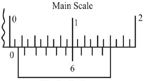
(1)
(2)
(3)
(4)
Show Answer
Correct answer: (3)
Solution:
The least count of the given vernier
Zero error
Observed reading,
Average
Vernier Callipers
3. The main scale, on a travelling microscope, has 20 divisions each between its different ‘centimeter marks’. The vernier scale, attached to it, has 50 divisions and these coincide with 49 divisions of the main scale.
The value of one vernier scale division, and the least count of this vernier, are equal, respectively, to
(1)
(2)
(3)
(4)
Show Answer
Correct answer: (4)
Solution:
There being 20 divisions, between the ‘centimeter marks’, the value of one main scale division is
Now 50 division, of the vernier, coincide with 49 division of the main scale. Hence value of one vernier scale division is
[Alternatively: Least count
Difficult
Vernier Callipers
4. A vernier scale set up, is used to find the internal diameter of a capillary tube. The basic details of this vernier are as follows:
No. of divisions on the vernier scale
No. of main scale divisions coinciding with these 50 divisions of the vernier scale
No. of divisions between the successive centimeter marks on the main scale
Zero error of this vernier scale
The readings, of the reference line, when the reference line, is in the positions

| Position | Main scale Reading | Coincident Vernier Division |
|---|---|---|
| A | 7 | |
| B | 3 |
The (measured) diameter, of this capilary tube, is
(1)
(2)
(3)
(4)
Show Answer
Correct answer: (3)
Solution:
Value of one M.S.D
No. of divisions on the vernier
Zero error
Total observed reading at end
Total observed reading at end
[Note: There is no need here to apply ‘zero correction’ to the readings at ends A and B. This is because we have to take the difference of the two readings. The identical correction applied to the two readings, would cancel out in the difference. This can be seen explicity as follows:
Corrected reading at end
Corrected reading at end
The same, as before (when the zero correction was not applied to the two readings).
Average
Vernier Callipers
5. The positions of the zeroes of the main scale and the vernier scale, when the jaws of the vernier just touch each other, is as shown in the figure.
This vernier is held vertical with the edge of its main scale just touching the mouth of a calorimeter and the end of its sliding strip just touching the bottom of the calorimter.
The reading of the main scale, at this positions is
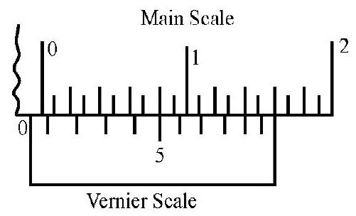
If the main scale is graduated up to
(1)
(2)
(3)
(4)
Show Answer
Correct answer: (1)
Solution:
The L.C of the vernier
Zero error
[Note: The (corrected) reading, observed this way, directly gives the depth of the calorimeter].
Average
Screw Guage
6. The positions of the ‘zeroes’ of the circular scale, with respect to the reference lines, (when the jaws are just put in contact), for two screw gauge
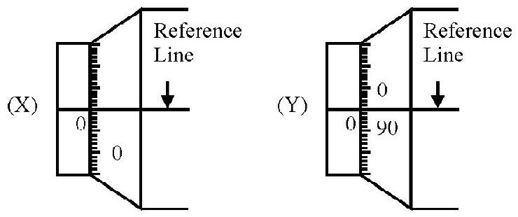
Screw gauge
‘Screw gauge
Four students reported the following basic information about the two ‘screw gauges’.
| Student | Screw Gauge X | Screw Gauge Y | ||||
|---|---|---|---|---|---|---|
| Pitch | Least Count | Zero Error | Pitch | Least Count | Zero Error | |
| A | ||||||
| B | ||||||
| C | ||||||
| D |
The complete correct reporting has been done by student
(1)
(2)
(3)
(4)
Show Answer
Correct answer: (1)
Solution:
For screw gauge
Pitch
Least count
Zero error
For screw gauge
Pitch
Least count
Zero error
Average
Screw Guage
7. The main scale, of a given screw gauge, has been graduated in ‘half millimeters’.
The moving jaw of this screw gauge advances through
The zero of the circular scale, coincides with the zero of the main scale when the moving face end just coincides with its fixed face end.
When a thin sheet is just held between the jaws of the screw guage, the main scale reads
(1)
(2)
(3)
(4)
Show Answer
Correct answer: (4)
Solution:
The pitch of the screw gauge
Main scale reading
Circular scale reading
Average
Screw Gauge
8. The basic information, about a given screw gauge, is as follows:
(i) Number of divisions on the circular scle
(ii) Distance moved, by the moving jaw, in 5 complete rotations
(iii) Position of the zero of the circular scale, when the two jaws just touch each other; as shown in the figure
When a wire is just held between the jaws of the screw gauge
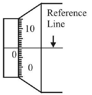
(a) Reading of the main scale
(b) No. of circular scale divison coinciding with the ‘reference line’
The radius, of this wire, equals
(1)
(2)
(3)
(4)
Show Answer
Correct answer: (1)
Solution:
Pitch
Zero error
Total observed reading
Radius of wire
Average
Screw Guage
9. The basic information, about a given screw gauge, is as follows:
(i) Least divison on the main scale
(ii) No. of divisons on the circular scale
(iii) Distance moved, on the main scale, when the screw is given 7 complete rotations
(iv) Circular scale division, coinciding with the line of graduated (reference) line, when the ‘jaws’, of the screw gauge, are just in contact
When a wire is just held in contact with the jaws of the screw gauge, the main scale reads
The zero error, and the corrected value of the radius of the wire, are equal, respectively, to
(1)
(2)
(3)
(4)
Show Answer
Correct answer: (2)
Solution:
Pitch
Zero error
Observed total reading
Corrected reading
Average
Screw Gauge
10. The least count, of a screw gauge, having 100 divisons, on its circular scale, equals 0.0005
The pitch and the ‘zero error’ of this screw gauge, are, respectively, equal to
(1)
(2)
(3)
(4)
Show Answer
Correct answer: (1)
Solution:
We have L.C
Total observed reading
Correct reading
Average
Simple Pendulum
11. The amplitude, of the oscillating bob of a simple pendulum, decreases form an initial value A to a value
The average rate of dissipation of energy, by the oscillating bob, is
(1)
(2)
(3)
(4)
Show Answer
Correct answer: (3)
Solution:
Initial Energy
Final energy
Difficult
Simple Pendulum
12. A student plots a graph between the ‘square of amplitude’, of the oscillating bob of a simple pendulum and ’time’. This graph is likely to be similar to the graph between the pair of variables, shown in the graph labelled as graph
[Note: For graph A, the values are for an ideal gas.
For graph B the displacement values are for a particle starting from rest and having a uniform acceleration.
For graph

For graph D,
(1)
(2)
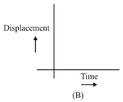
(3)
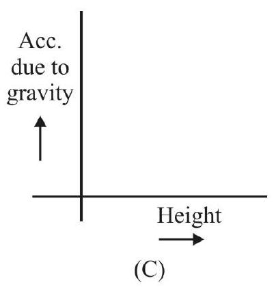
(4)
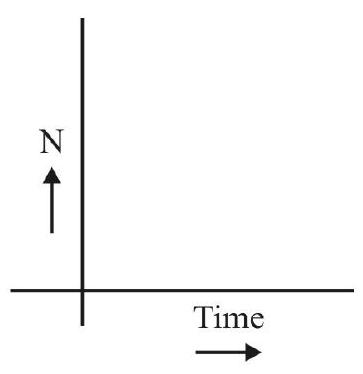
Show Answer
Correct answer: (4)
Solution:
The ‘square of amplitude’, of the bob, is likely to decay exponentially with time
For graph
For graph
For graph
For graph
Hence it is only graph in which the variation is an ’exponential decay’ with time.
Average
Simple Pendulum
13. The (small) amplitude, of the oscillating bob, of a simple pendulum becomes
(1)
(2)
(3)
(4)
Show Answer
Correct answer: (2)
Solution:
The energy of the bob
Final energy
Average
Simple Pendulum
14. When a simple pendulum executes small amplitude oscillations in a medium (like air), its amplitude decreases, quite slowly
(1) with time (in a linear way) but its time period remains completely independent of its amplitude.
(2) with time (in a non-linear way) but it time period remains completely independent of its amplitude.
(3) with time (in a non-linear way) and its time period shows a slight increase compared to its time period in free space.
(4) With time (in a linear way) and its time period shows a slight decrease compared to its time period in free space.
Show Answer
Correct answer: (3)
Solution:
The oscillations, of a pendulum bob, in a medium (like air) are damped oscillations. For such damped oscillations, the amplitude decreases exponentially with time, i.e., its decrease is a non-linear one.
The time period, for such damped oscillations, is (slightly) more than its the time period in free space.
Average
Using the Principle of Moments to Find the Mass of a given Meter Scale
15. A meter scale, and a system of three ‘weights’, is set up as shown. The mass of the ‘weight’, labelled as

(1)
(2)
(3)
(4)
Show Answer
Correct answer: (2)
Solution:
Taking moments about the midpoint,
or
Average
Using the Principle of Moments to Find the Mass of a given Meter Scale
16. A meter scale and two objects, of (known) masses
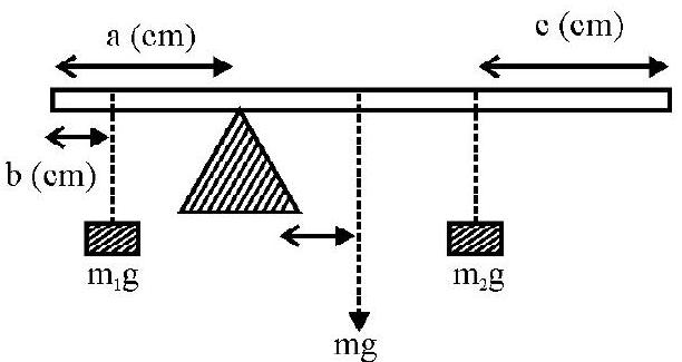
(1)
(2)
(3)
(4)
Show Answer
Correct answer: (1)
Solution:
Total clockwise moments about the wedge
Total anticlockwise moments about the wedge
or
Average
Young’s Modulus
17. A meter scale gets balanced at its
(1)
(2)
(3)
(4)
Show Answer
Correct answer: (3)
Solution:
Let
In the second case, when the object of unknown mass
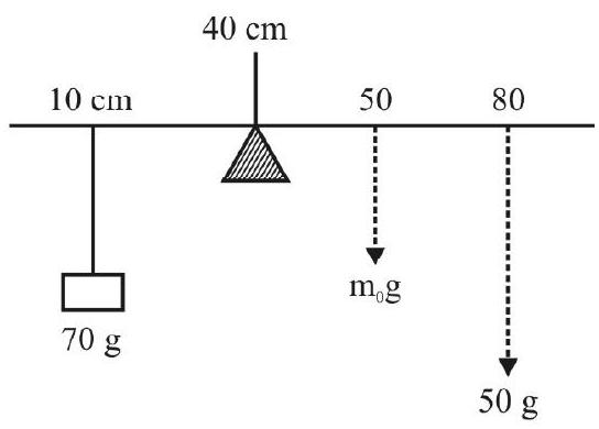
Average
Young’s Modulus
18. A force, F, applied to the experimental wire in a Searle’s apparents set up, increases its length by an amount
If the diameter of this experimental wire were to be doubled and the force applied increased to
(1)
(2)
(3)
(4)
Show Answer
Correct answer: (4)
Solution:
We have,
Also
or
Average
Young’s Modulus
19. A rod of a material, of length
When the temperature of the rod increases by
(1)
(2)
(3)
(4)
Show Answer
Correct answer: (2)
Solution:
When the temperature increases by
The corresponding longitudinal strain is
If Y be the Young’s modulus of the material of the rod, the stress developed is given by
Stress
Average
Poisson’s Ratio
20. A wire, of length
(1)
(2)
(3)
(4)
Show Answer
Correct answer: (1)
Solution:
The (original) volume of the wire is
When the length of the wire increases by an amount
We thus have
The Poisson’s ratio,
Difficult
Young’s Modulus
21. The breaking stress, for a (light) wire of a given material, is
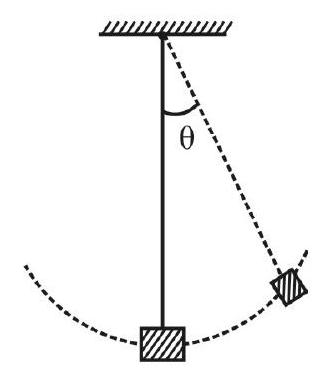
(1)
(2)
(3)
(4)
Show Answer
Correct answer: (4)
Solution:
When the wire is displaced through an angle
The increase in P.E., of the mass, is Mgh. Hence if
At the mean position, the total tension, developed in the wire, would be
The corresponding stress is
This would just equal the breaking stress if
or
or
Average
Surface Tension
22. It is well known that water forms a concave meniscus while mercury forms a convex meniscus when they are present in a glass tube. This is because the
(1) Density of mercury is more than that of glass while water has a density less than that of glass.
(2) Force of cohesion, between water molecules is more than the force of adhesion between water and glass; the reverse in true for mercury.
(3) Force of cohesion, between water molecules, is less thatn the force of adhesion between water and glass; the reverse is true for mercury.
(4) Excess of pressure, inside a water drop of radius
Show Answer
Correct answer: (3)
Solution:
The shape of the meniscus, of a given liquid, in a given container, is determined primarly by the comparative magnitudes of the relevant forces of cohesion and adhesion.
For liquids (like water), the force of cohesion between liquid molecules, is less than the force of adhesion between the liquid molecules and the molecules of the walls of the container (glass). In such a case, the liquid forms a concave meniscus.
The reverse is true for mercury put in a glass tube. In such a case the liquid forms a convex meniscus.
[Note: Option (4) is incorrect; the excess pressure
Average
Capillary Rise
23. Two liquids, (having surface tensions
(1)
(2)
(3)
(4)
Show Answer
Correct answer: (2)
Solution:
We know that
For the two given liquids
and
or
Average
Capillary Rise
24. A given liquid rises to a height
(1) will start over flowing through the capillary tube.
(2) will have a readjusted value of its surface tension for which the rise is equal to
(3) will readjust its angle of contact, with the walls of the container, to a new value, say
(4) will readjust its angle of contact, with the walls of the container, to a new value, say
Show Answer
Correct answer: (3)
Solution:
The liquid will not overflow as that would lead to a violation of the principle of conservation of energy. For the rise (h) of a liquid, in a capillary tube of radius,
For a capillary tube, of insufficient height, the liquid, readjusts its angle of contact with the walls of the container, so that
[Note: The liquid does not readjust its surface tension to a new value].
Difficult
Capillary Rise
25. Two liquids (say
(1)
(2)
(3)
(4)
Show Answer
Correct answer: (4)
Solution:
We know that
From the given data, we then have
Average
Terminal Velocity
26. A drop of a liquid, of radius
(1)
(2)
(3)
(4)
Show Answer
Correct answer: (2)
Solution:
Let
We then have
The relation, between the terminal velocity and the radius of the drop, is given by
or
Difficult
Terminal Velocity
27. A drop of a liquid, of a given radius, falls vertically through a given viscous medium. The pair of graphs, that respresent the variation of velocity (v), and acceleration (a) of the falling drop, with time, is the pair marked as pair
(1)
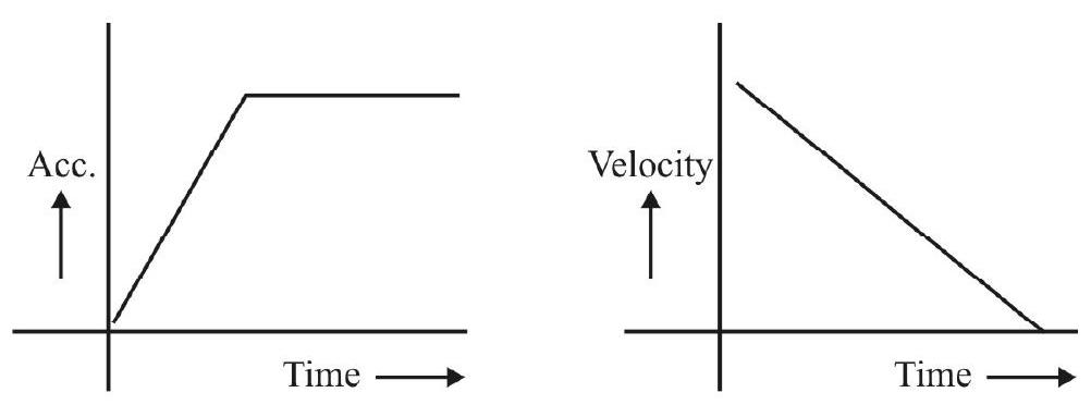
(2)
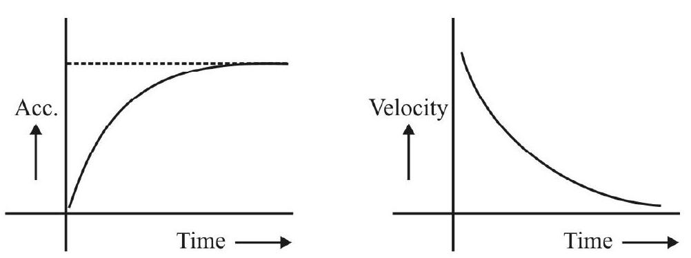
(3)
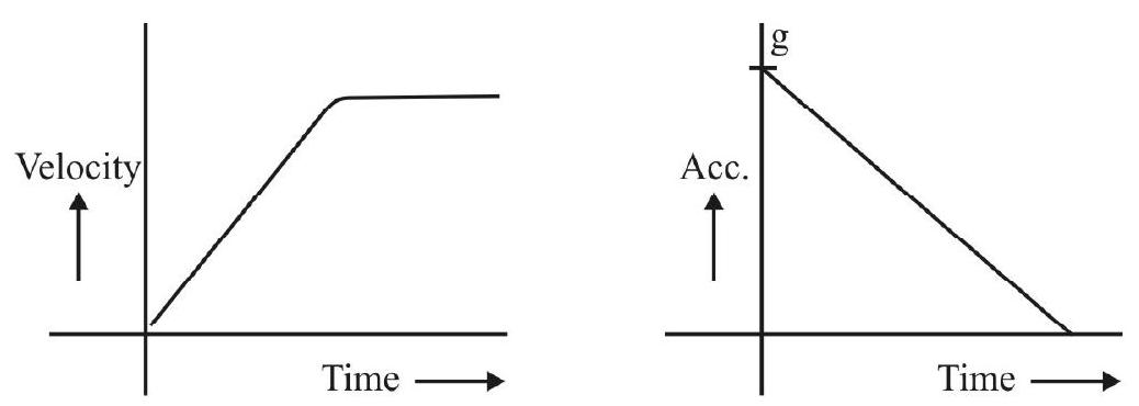
(4)
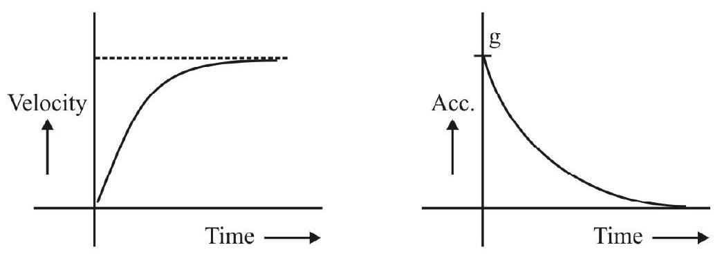
Show Answer
Correct answer: (4)
Solution:
As the drop falls vertically through the viscous medium, its velocity keeps on increasing with time. This, in turn, increases the viscous force acting on it so that its acceleration keeps on decreasing with time. When the viscous force becomes large enought to balance the net downward force, the acceleration of the drop becomes zero. Its velocity than remains constant (with time) at a value called the terminal velocity of the graph.
This variation of velocity and acceleration, with time, is non-linear because of the non-uniform accleration of the falling drop. The pair (D) shows the variations in their correct form.
Average
Terminal Velocity
28. A drop of a liquid, of density
The terminal velocities (
(1)
(2)
(3)
(4)
Show Answer
Correct answer: (3)
Solution:
We know that
and for the second drop,
Difficult
Stoke’s Law
29. A spherical ball, of mass
(1)
(2)
(3)
(4)
Show Answer
Correct answer: (4)
Solution:
Let the velocity of the ball be
The acceleration,
or
or
Average
Newton’s Law of Cooling
30. To do an experimental verification of Newton’s law of cooling, we need to take the ’temperature’ vs ’time’ readings, of a hot body, kept in given surroundings. An appropriate choice, of the ‘hot body’ and the ‘surroundings’, would then be:
(1) [A hot metal sphere]; and [a ‘closed enclosure’].
(2) [A hot metal sphere]; [a stone plate to hold the sphere and kept in an uncovered enclosure].
(3) [An uncovered calorimeter containing hot water that is constantly being stirred]; [a slab on an open window or a table under a fan].
(4) [A fully covered calorimeter containing hot water]; [a corner of the room away from any open window or a fan].
Show Answer
Correct answer: (3)
Solution:
Newton’s law of coolings holds for the cooling of a hot body, primarily by convection. It can then be valid even for quite a large difference of temperature between the hot body and the surroundings.
The ‘set-up’, suggested in option (3), is most likely to ensure that the whole of the hot body cools primarily by convection. Hence it is the appropriate choice for verifying Newton’s law of cooling.
Difficult
Cooling Time
31. A hot body, initially at a temperature
(1) 2
(2)
(3)
(4)
Show Answer
Correct answer: (3)
Solution:
We know that
or
and (ii)
Average
Graph of Increase of Temperature with Time
32. A given object (initially at a temperature
(1)
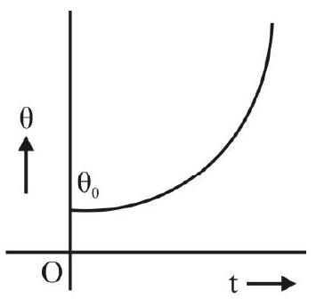
(2)
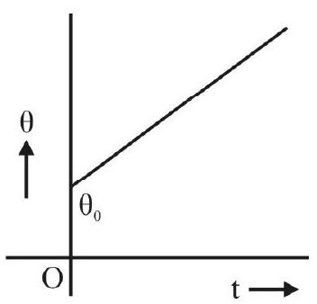
(3)
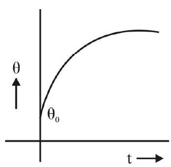
(4)
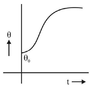
Show Answer
Correct answer: (2)
Solution:
Let the temperature of the object (mass
Average
Experimental Skills
33. A hot body, initially at a temperature
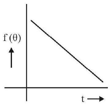
(1)
(2)
(3)
(4)
Show Answer
Correct answer: (4)
Solution:
As per Newton’s law of cooling
or
or
Hence
Easy
Speed of Sound in Air
34. A student sets up the speed of sound in air apparatus for finding the velocity of sound in air, at the room temperature. Using a tuning fork, of frequency
(1)
(2)
(3)
(4)
Show Answer
Correct answer: (3)
Solution:
We have
and
The velocity,
[Note: It is only this formula for
Average
Speed of Sound in Air
35. The experiment, using a resonance tube set-up, was carried out in a room at a temperature
From these observations, one can say that the velocity of sound, in air, at
(1)
(2)
(3)
(4)
Show Answer
Correct answer: (2)
Solution:
We have
and
We also have
Average
Speed of Sound in Air
36. Two students, working in the same laboratory, do the experiment on finding the velocity of sound using the ‘resonance tube column apparatus’. They used tubes of diameters
(1)
(2)
(3)
(4)
Show Answer
Correct answer: (3)
Solution:
We know that
and
Also end correction
and
Difficult
Speed of Sound in Air
37. A student did the experiment on finding the speed of sound (say
(1)
(2)
(3)
(4)
Show Answer
Correct answer: (1)
Solution:
We know that
or
Also
or
Also
We thus have
and
Average
Specific Heat Capacity
38. A given liquid wasknown to be (chemically) non-reactive with water; a mass,
(1)
(2)
(3)
(4)
Show Answer
Correct answer: (4)
Solution:
Heat is lost only by the hot liquid. Hence heat lost
Heat is gained both by the second calorimeter and the water contained in it.
Hence heat gained
Putting heat gained
Difficult
Specific Heat Capacity
39. When a given amount of heat (say
(i) mass
(ii) mass
(1) zero
(2)
(3)
(4)
Show Answer
Correct answer: (2)
Solution:
We have
Similarly
We also have
Difficult
Specific Heat Capacity
40. A given solid rectangular bar
and
The heat needed to raise the temperature of this bar by an amount,
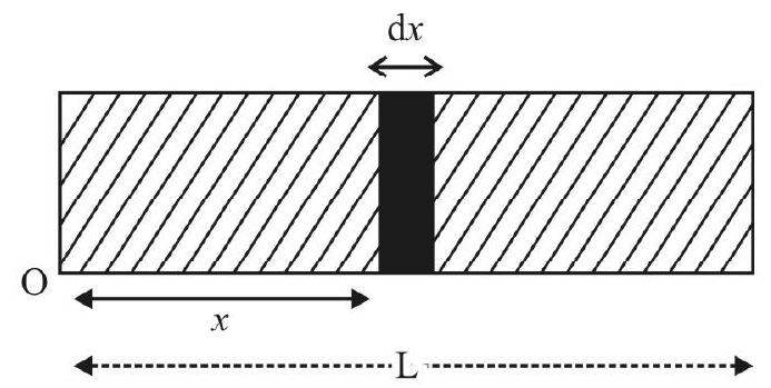
(1)
(2)
(3)
(4)
Show Answer
Correct answer: (2)
Solution:
The mass, dm, of a segment of the bar, of length
The specific heat capacity, of this segment, is
Hence the heat needed to raise its temperature, by an amount
Hence the total heat needed is
The total mass of the bar, is
Difficult
Loss of Heat by a Hot Solid
41. It is given that the rate of loss of heat by a substance, at any temperature, is proportional to the difference between that temperature and the temperature of the surroundings. A solid, of mass
The ratio of the times, taken by this solid, in cooling (i) from
(1)
(2)
(3)
(4)
Show Answer
Correct answer: (3)
Solution:
The (small) amount of heat (
We are given that
If follows that
(i)
and (ii)
Difficult
Meter Bridge
42. In a metre bridge experiment to find the resistance of a uniform wire of length
(1)
(2)
(3)
(4)
Show Answer
Correct answer: (2)
Solution:
Let
The effective length is
Now,
Average
Meter Bridge
43. A metre bridge circuit, with resistance
(1)
(2)
(3)
(4)
Show Answer
Correct answer: (4)
Solution:
Given
When
When
Since balancing length remains same,
or
or
or
or
Alternatively: Since the balacing length is the same, potential drops across the gaps remain the same. Therefore, the ratio of resistances would be the same along individual paths.
or
Easy
Meter Bridge
44. In a metre bridge experiment, to determine the specific resistance (
(1)
(2)
(3)
(4)
Show Answer
Correct answer: (4)
Solution:
The formula for
Difficult
Ohm’s Law
45. While performing the experiment, to find the resistance
If the milliammeter read
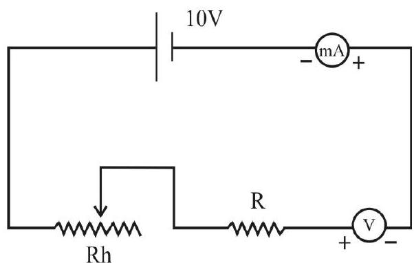
(1)
(2)
(3)
(4)
Show Answer
Correct answer: (2)
Solution:
In series also, a voltmeter will still read the potential difference across its terminals.
or
The resistance, due to the rheostat, is half of its total resistance of
Total potential applied
Therefore, the value of
Average
Ohm’s Law
46. While performing the experiment on Ohm’s law, a student plotted the V-I graphs for two resistances, individually and for their series and parallel combinations. The four plots are marked A, B, C and D in the graph shown below. The values of the individual resistances in ohm, are approximately
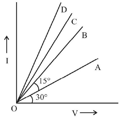
(1) 1 and
(2) 1 and
(3) 1 and 0.732
(4)
Show Answer
Correct answer: (3)
Solution:
Since
A is maximum and the value of
This must be the resistance for the series combination. Since the resistance is the least for
Therefore graphs B and C are for the individual resistances.
B graph representing one of the resistances, has its slope as unity. Hence this resistance is
Hence the two resistances are
Average
Ohm’s Law
47. Using the Ohm’s circuit, for determination of resistnace of a wire made of an alloy of constant temperature coefficient of resistance
(1)
(2)
(3)
(4)
Show Answer
Correct answer: (2)
Solution:
The variation of
Hence we have
Easy
Potentiometer
48. Which of the following statements is incorrect regarding the use of the high resistance in the potentiometer circuit?
(1) It protects the galvanometer from being damaged due to high current.
(2) Its value does not play any role in the determination of null point.
(3) It must always be necessarily connected just before the galvanometer to prevent high current entering the galvanometer.
(4) It can be short circuited when the jockey, moved along the wire, approaches the null point position.
Show Answer
Correct answer: (3)
Solution:
(1) The galvanometer circuit can have large current when the jockey is pressed near the extreme ends of the poteniomeer wire due to the large potential difference across the wire, far away from the null point. Since the galvanometer is highly sensitive, it might get damaged due to this high current. Ahigh resistance will reduce this current and protect the galvanometer. Hence (1) is a correct statement.
(2) At the null point the deflection in the galvanometer is zero as the current is zero. So the value of this high resistance does not decide the position of the null point, it only decreases the deflection when jockey is pressured at other points. So (2) is also a correct statement.
(3) Since a resistor only obstruct the flow of charge, the position of the resistor can be anywhere in the series part of the circuit. That means, the high resistance can be before, or after, the galvanometer. In either case the current gets reduced. So (3) is an incorrect statement (i.e. (3) is the correct answer to the question).
(4) When we approach the null point, the current through the galvanometer approaches zero or the deflection becomes almost zero. Here if we short circuit the high resistance, the deflection becomes obviously more, but the current will not to so high as to damage the galvanometer. Instead the short circuit of the high resistance will enable us to find the null point accurately. So (4) is also a correct statement.
Average
Potentiometer Internal Resistance
49. In a potentiometer experiment the following circuit arrangement is used.
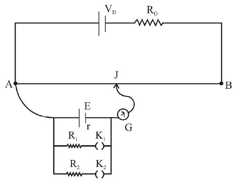
When the key
(1)
(2)
(3)
(4)
Show Answer
Correct answer: (3)
Solution:
Let
Here
But
Let
Then
But
Dividing (1) by (2), we get:
or
or
Difficult
Potentiometer - Comparison of emfs
50. A potentiometer wire
The balacing length, measured from
(1)
(2)
(3)
(4)
Show Answer
Correct answer: (1)
Solution:
Given
Now, let
Let I be the current through the wire, which must be the same for both the halves.
By using the principle of potentiometer,
and
Difficult
Potentiometer Application
51. For the potentiomeer circuit, set up as shown, the potential gradient, across the potentiometer wire,
Assuming that the current value, as obtained through the potentiometer readings, is the correct value of current, the percentage error, in the reading of the ammeter, equals
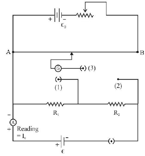
(1)
(2)
(3)
(4)
Show Answer
Correct answer: (1)
Solution:
When the gap between points (1) and (3) is plugged in, we have
Potential drop across
Current read by the ammeter
Similarly, with the gap between points (2) and (3) plugged in, we get the percentage error in ammeter reading as
The percentage error can thus have either of the values given by expressions (1) and (2).
Difficult
Galvanometer Resistance
52. A galvanometer, of unknown figure of merit
The experimental values of
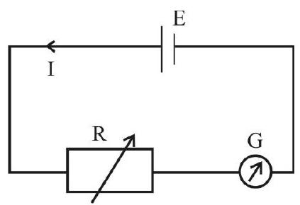
(1) Slope of the graph
(2)
(3) Ratio of y-intercept to the slope of the graph
(4) Product of y-intercept and the slope of the graph
Show Answer
Correct answer: (3)
Solution:
From the circuit, the value of I can be written as:
or
or
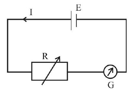
Since
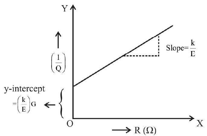
Now,
Easy
Galvanometer – G and K
53. In the galvanometer experiment, the values of
He would use the resistor:
(1)
(2)
(3)
(4)
Show Answer
Correct answer: (4)
Solution:
To convert the galvanometer in to a voltmeter, he has to connect a series resistor
The value of
Here,
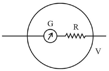
The colour code corresponding to this
Brown, Violet, Red.
Therefore
Easy
Half Deflection Method
54. While performing the galvanometer experiment using half deflection method, a student got almost the same value for
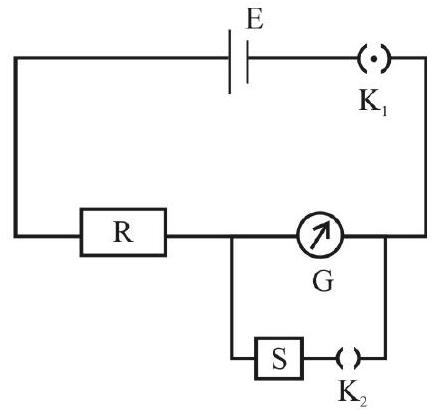
(1) The resistance box in which
(2) Resistance G is very low
(3) In half-deflection method, current gets divided between
(4) The internal resistance of the d.c source varies with current flow
Show Answer
Correct answer: (3)
Solution:
Here, the galvanometer is a very sensitive device. The current flowing in it should be very low. So
The formula for
Since
This shows that,
Difficult
Finding the Resistance of Galvanometer
55. For the circuit shown here, the galvanometer deflection equals (i) 15 divisons when the key
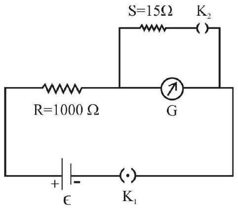
(1)
(2)
(3)
(4)
Show Answer
Correct answer: (2)
Solution:
With the key
When the key
We are given that
Average
Focal Length of Concave Mirror
56. In the experiment to find the focal length of a concave mirror, using parallex method, a student placed the object pin at a point so at to obtain an enlarged real image. He used an image pin in order to locate the position of this real image of the object pin, by trying to remove the parallex between the two. Checking for parallex, he observed that the image of the object pin moved through greater distance than the image pin, with respect to the edge of the mirror, when he moved his eye. The position, across the optical bench (with respect to the present position of the image pin), of the image (of the object-pin) is:
(1) Closer to his eyes.
(2) Closer to the centre of curvature of the mirror.
(3) between the image pin and the centre of curvature of the mirror.
(4) At the position of the object pin.
Show Answer
Correct answer: (1)
Solution:
It is obvious that more the relative distance moved closer will be the object observed (here the image of the object-pin), with respect to the other.Hence the image (of the object pin) is closer to his eyes.
Average
Focal Length of Convex Lens
57. While using the displacement method, for determination of focal length of a convex lens, a student placed the object pin at
(1)
(2)
(3)
(4)
Show Answer
Correct answer: (2)
Solution:
The formula for
Average
Focal Length of Convex Lens
58. In the experiment to determine the focal length of a convex lens, using the method of parallex, the following observation were recorded by a student. Which of the observations is possibly not taken correctly by the student?
| Sl. No. | Position of the object |
Position of Lens |
Position of Image |
|---|---|---|---|
| 1. | 25 | 50 | 66.7 |
| 2. | 30 | 50 | 70.0 |
| 3. | 35 | 50 | 80.0 |
| 4. | 38 | 50 | 88.0 |
| 5. | 20 | 50 | 65.0 |
| 6. | 15 | 50 | 64.0 |
(1) S. No. 6
(2) S. No. 5
(3) S. No. 4
(4) S. No. 3
Show Answer
Correct answer: (3)
Solution:
Obtaining the values of
| SI. No. | Position of the object |
Position of Lens |
Position of Imagc |
|||
|---|---|---|---|---|---|---|
| 1. | 25 | 50 | 66.7 | 25 | 16.7 | 10.0 |
| 2. | 30 | 50 | 70.0 | 20 | 20.0 | 10.0 |
| 3. | 35 | 50 | 80.0 | 15 | 30.0 | 10.0 |
| 4. | 38 | 50 | 88.0 | 12 | 38.0 | 9.1 |
| 5. | 20 | 50 | 65.0 | 30 | 15.0 | 10.0 |
| 6. | 15 | 50 | 64.0 | 35 | 14.0 | 10.0 |
Clearly, observation at Sl. No. 4, has not been taken correctly.
Average
Focal Length of Convex Lens
59. A convex lens, of focal length,
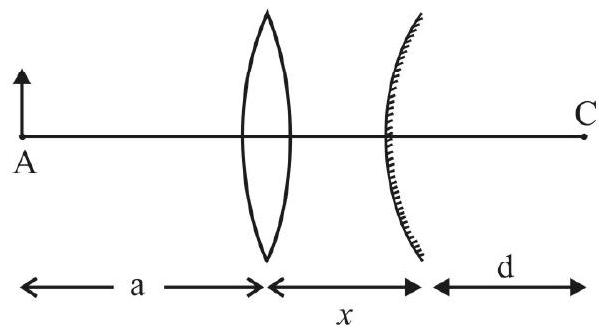
(1)
(2)
(3)
(4)
Show Answer
Correct answer: (3)
Solution:
The image of the object, put at A, coincides with the object itself. This implies that the rays, redfracted by the convex lens, are incident normally on the convex mirror. Hence the image, formed by the convex lens alone, is at a distance
This gives
We are given that
Hence
Average
Redfraction of Lightly Prism
60. A ray of light is incident at grazing incidence on one face of an equilateral prism made from a transparent material of redfractive index
(1)
(2)
(3)
(4)
Show Answer
Correct answer: (1)
Solution:
For the ray, incident at grazing incidence, on one face, the corresponding angle of redfraction,
If angle of incidence, at the second face, is
Also, if
Difficult
Refractive of Light Through a Prism
61. A ray of light, incident on the face
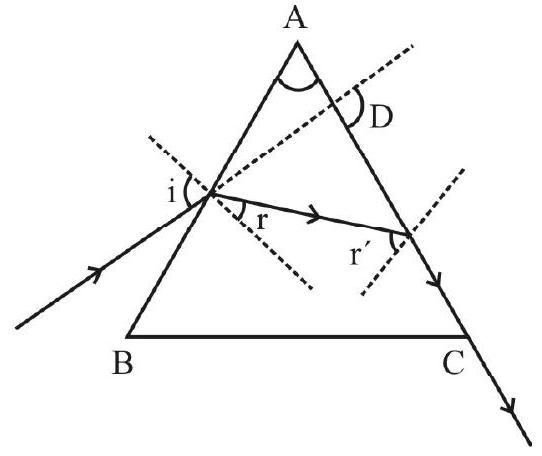
(1)
(2)
(3)
(4)
Show Answer
Correct answer: (4)
Solution:
It is clear that the angle of emergence, at the face
We have
Also,
Again, by Snell’s law,
Difficult
Refraction of Light by Prism
62. Light, incident on the face
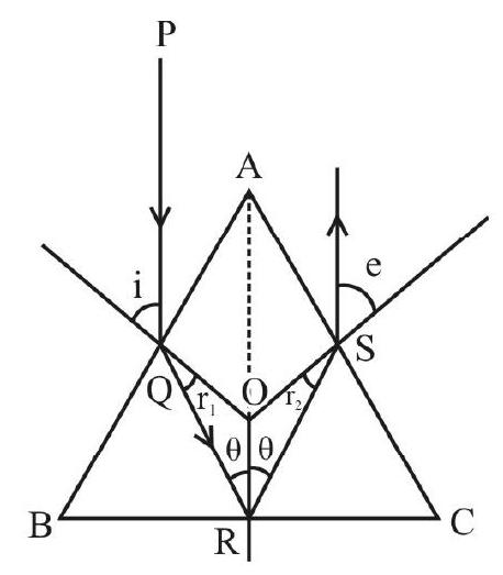
(1)
(2)
(3)
(4)
Show Answer
Correct answer: (2)
Solution:
Since there is total internal reflection at the face
From cyclic quadrilaterial
But
Difficult
Real and Apparent Height
63. A transparent oil, of redfractive index
A tiny shining metal ball, lying at the bottom of the container, is viewed from above. Its ‘apparent height’, above the bottom of the container equals, a dfraction,
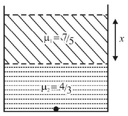
(1) 0.27
(2) 0.30
(3) 0.32
(4) 0.35
Show Answer
Correct answer: (1)
Solution:
The depths, of the two liquids, are in the ratio
Apparent depth of the top layer
Apparent depth of the bottom layer
Difficult
Refractive Index
64. A tiny air bubble, trapped inside a glass cube of side a, appears to be at distances
(1)
(2)
(3)
(4)
Show Answer
Correct answer: (4)
Solution:
The apparent distance, of the air bubble from the first face, is
Hence
For the opposite face, the real distance, of the air bubble, would be (a-x). Hence
Dividing, we get
Average
‘Real and Apparent Depth’
65. Three layers of three different transparent media (of redfractive indices
(1)
(2)
(3)
(4)
Show Answer
Correct answer: (3)
Solution:
The apparent depth, of a layer of a medium of redfractive index
Easy
P–N Junction Diode
66. The reverse saturation current in a
(1) increases with increase in applied voltage
(2) decreases with increase in applied voltage
(3) increases with increase in temperature
(4) decreases with increase in temperature
Show Answer
Correct answer: (3)
Solution:
Reverse saturation current depends on the rate of generation of electron hole pair, which is independent of the applied voltage.
In fact,
Hence
Average
P–N Junction Diode
67. The slope of
(1) Planck’s constant
(2) Boltzman constant (Correct)
(3) Reverse saturation current (Incorrect)
(4) Mobility of minority charge carriers
Show Answer
Correct answer: (2)
Solution:
We have
It can give value of
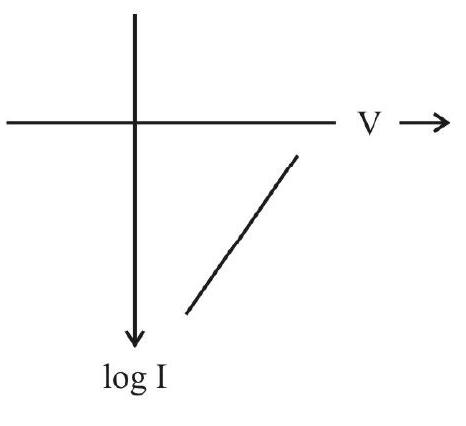
Easy
P–N Junction Diode
68. The depletion region in a
(1) Ionized donor impurities
(2) Ionized acceptor impurities
(3) Immobile charge carriers
(4) Mobile charges carriers
Show Answer
Correct answer: (4)
Solution:
There is a recombination of electrons and holes in the deplections region. Hence the charge carriers, in this region, are immobile.
Easy
69. The motion of charge carriers, across the potential barrier, in a forward and reverse biased
(1) Drift, diffusion
(2) Diffusion, drift
(3) Drift in both cases
(4) Diffusion in both cases
Show Answer
Correct answer: (2)
Solution:
The charge carriers, diffuse across the junction during the forward biasing of a
During reverse biasing, the motion of charge cariers, is due to their drift.
Average
Zener Diode
70. In the circuit given below, the Zener voltage is maintained at
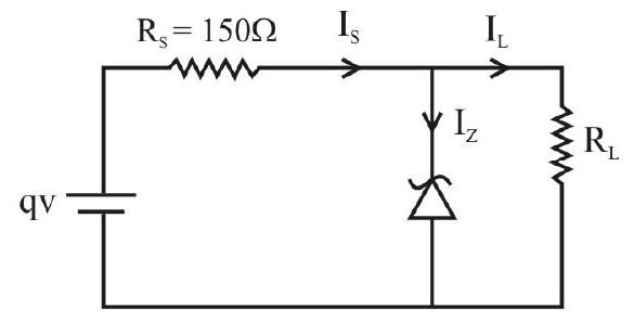
(1)
(2)
(3)
(4)
Show Answer
Correct answer: (4)
Solution:
We have,
Average
Zener Diode
71. In the circuit given below, the Zener voltage is
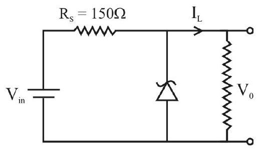
(1) always be
(2) lie between
(3) equal
(4) lie between
Show Answer
Correct answer: (4)
Solution:
The equivalent circuit diagram gives
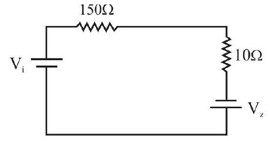
If
If
Easy
Doping of a Diode
72. It will be correct to say that,
(1) A lightly doped diode has a thin deplection layer and a higher breakdown voltage (Incorrect)
(2) A heavily doped diode has a thin deplection layer and a lower breakdown voltage (Correct)
(3) A lightly doped diode has a wide deplection layer and a lower breakdown voltage (Incorrect)
(4) A heavily doped diode has wide deplection layer and a higher breakdown voltage Incorrect)
Show Answer
Correct answer: (2)
Solution:
The width of the deplection layer, as well as the barrier potential across the junction, both decrease with an increase in the extent of doping, of the
Easy
Junction Transistor
73. The input resistance, of a pnp transistor, in its common emitter configuration, is given by,
(1)
(2)
(3)
(4)
Show Answer
Correct answer: (1)
Solution:
The input resitance is defined as
Easy
Junction Transistor
74. In a bijunction transistor, the base region is,
(1) Lightly doped so that recombination is more
(2) Lightly doped so that recombination is less
(3) Heavily doped so that recombination is more
(4) Heavily doped so that recombination is less
Show Answer
Correct answer: (2)
Solution:
The base region is kept thin and is also lightly doped. This is to ensure that the charge carriers, from the emitter, cross over (without any significant recombination) and get collected in the collector region.
Average
Junction Transistor
75. One of the differences/similarity, in the operation of a transistor amplifier, and a step-up transformer, is
(1) In transistor, if voltage increases, current also increases, in step-up transformer, if voltage increases, current decreases
(2) In transistor, if voltage increases, current increase; in step-up transformer, if voltage increasee, current increases
(3) In both of them, if voltage increases, current also increases
(4) In both of them, if voltage increases, current decreases
Show Answer
Correct answer: (1)
Solution:
The transistor can bring about an increases in voltage along with an increase in current. This is because the increased power, in the ‘output’ of a transistor, comes at the expense of the power supplied by the biasing battery.
In a step-up transformer, there is no such power source. Hence the ‘output’ power - even in the case of an ideal transformer - can at best be equal to the ‘input’ power. The increase in voltage, here, is accompnied by a decrease in current, and vice-versa.
Average
‘Current Gain’ in a Transistor
76. For a given transistor, if
(1) 0.0
(2) 1.0
(3) 200
(4) 201
Show Answer
Correct answer: (2)
Solution:
This is so because
’
Average
Multimeter Use
77. While checking a diode with a digital multimeter, set to its ‘diode’ symbol, a good diode is expected to show.
(1)
(2)
(3)
(4) 1 in both forward and reverse polarity
Show Answer
Correct answer: (3)
Solution:
In forward bias, it shows voltage drop across the diode which is small,
Easy
LED
78. The voltage drop, across a LED, when connected in forward bias configuration to a multimeter, is,
(1) 0.5 to
(2) 1.5 to
(3) 0.5 to
(4) 1.5 to
Show Answer
Correct answer: (2)
Solution:
The voltage drop, across LED, in the forward bias configuration, is in the range of
Easy
Identification of a Given Device
79. A small device has a yellow colored capsule top and has 220 written on it. There is no + or - sign on it. This device is likely to be
(1) Electrolyte capacitor of value
(2) Electrolytc capacitor of value
(3) Ceramic capacitor of value
(4) Ceramic capacitor of value
Show Answer
Correct answer: (4)
Solution:
The given description matches a ceramic capacitor of value
Average
Identifying the Base of a Transistor
80. If negative probe of a multimeter is placed
(1) a low resistance
(2) a high resistance
(3) zero resistance
(4) (1-) reading
Show Answer
Correct answer: (1)
Solution:
When the negative probe of a multimeter (adjusted to work as an ohm meter) is placed on the base of a


