UNIT 14 ELECTROMAGNETIC INDUCTION AND ALTERNATING CURRENTS
Learning Objectives
After going through this, unit you will be able to understand, appreciate and apply the following concept:
- Understand the methods, or ways, to induce emf in a coil.
- Understand the Faraday’s law of induction and Lenz’s Law.
- Calculate emf, current and magnetic flux using Faradays’ Law.
- Explain the physical meaning of Lenz’s Law.
- Derive the formula for motional emf and power spent by external agency in moving a coil with constant velocity.
- Explain the magnitude and direction of an induced eddy current, and the effect this will have on the object it is induced in.
- Describe the several applications of eddy currents.
- Explain the self induction and back emf.
- Calculate the inductance, energy stored and emf generated in a coil/ inductor.
- Explain the mutual induction between the neighbouring coils.
- Calculate the mutual inductance of coaxial solenoids.
- Sketch (draw phasor diagrams) voltage and current versus time in simple inductive, capacitive and resistive circuits.
- Calculate the reactance, impedance, current and voltage in simple series a.c. circuits having L, C and R.
- Derive the phase angle, resonant frequency, power, power factors in series LCR circuit.
- Explain the significance of series resonant circuit, resonant freqeuncy and quality factor.
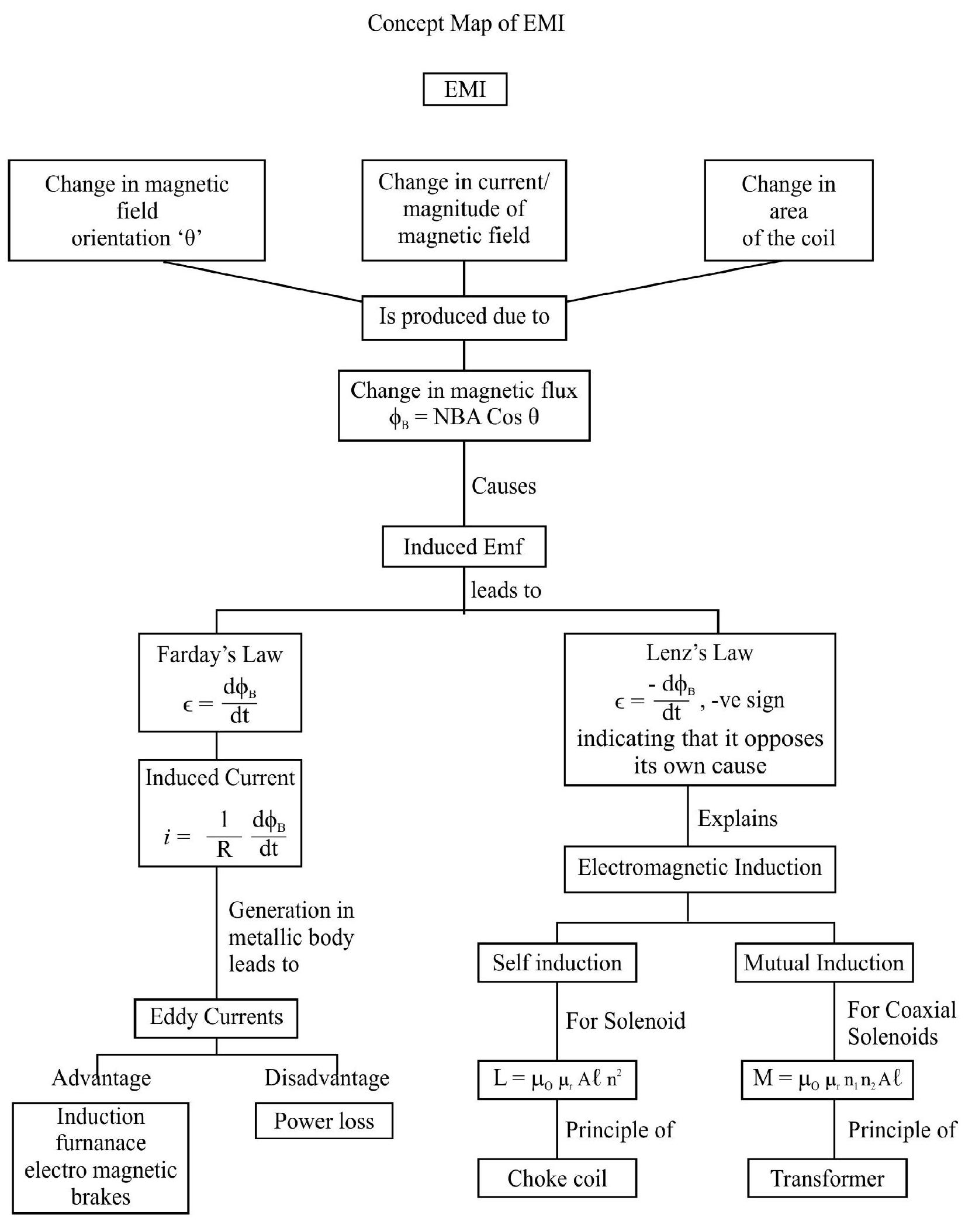
Electromagnetic Induction
Magnetic Flux
The number of magnetic field lines, or magnetic flux ’
where
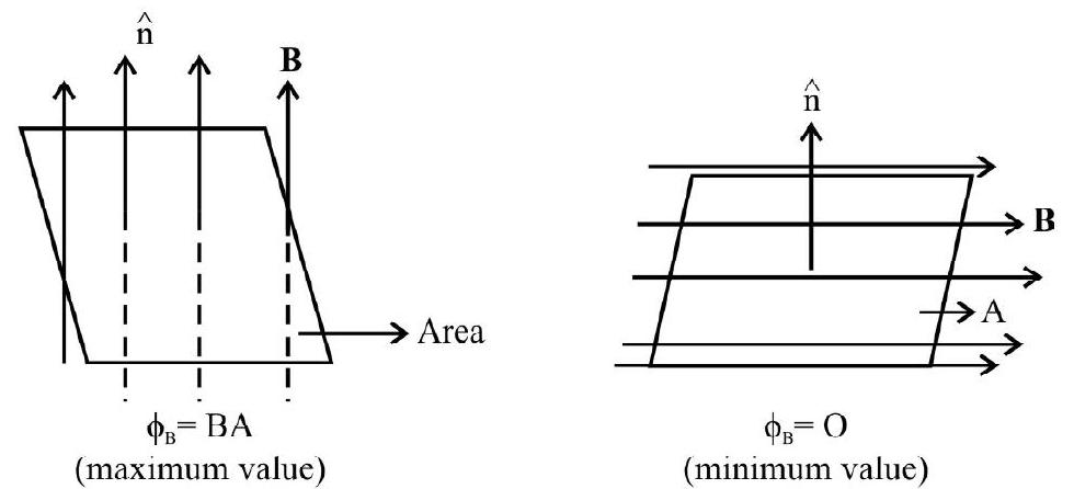
The figures, given above, show the positions (of the area A, with respect to the direction of a uniform magnetic field) for which the magnetic flux, linked with the area, has its
(i) maximum value
(ii) minimum value
Electromagnetic Induction
We knwo that moving electric charges, or currents, can produce magnetic fields. Is the conserve effect possible? Can moving magnets produce electric currents? In the year 1830, Faraday conducted many experiments to demonstrade that electric currents can be induced in closed coils when they are present in a changing magnetic field or when changing the magnetic flux, linked with them, is made to change.
From the experiemental observations of Faraday, it was concluded that whenever the number of magnetic field lines or magnetic flux, passing through a coil changes, an emf is induced in that coil. If the circuit is closed, a current flows through it. The emf, and the current so produced, are called. ‘induced emf’ and ‘induced current’ respectivley. They last only as long as the (linked) magnetic flux is changing. This phenomenon is now known as ’electromagnetic induction’.
Ways of Changing the (Linked) Magnetic Flux
The magnetic flux, through a circuit, may be changed in a number of ways. This can be done (i) by moving a magnet relative to the circuit (ii) by changing the current in a neighbouring circuit (iii) by changing the current in the same circuit and (iv) by rotating a coil in a uniform magnetic field.
Let us no consider two experiments demonstrating the phenomenon of electromagnetic.
Experiment-1 :
When a bar magnet is pushed towards or pulled away, from the coil, the pointer in the galvanometer deflects. This indicates the presence of electric current in the coil.
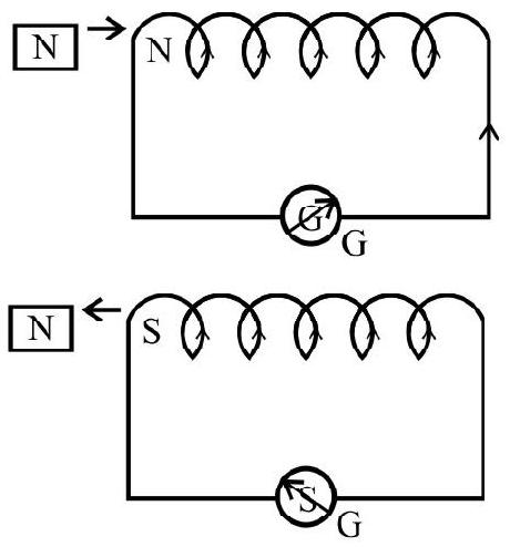
The deflection, in the two cases are, however, in opposite senses.
- It is also observed that faster the motion of the magnet, larger the deflection.
- When the bar magnet is held fixed and the coil is moved towards or away from the magnet, similar effects are observed.
- This shows that it is the existence of a relative motion, between the magnet and the coil, that is responsible for inducing electric current in the coil.
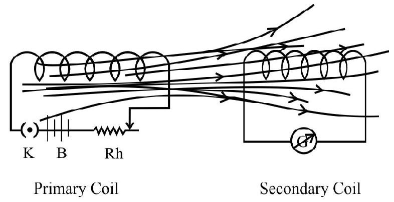
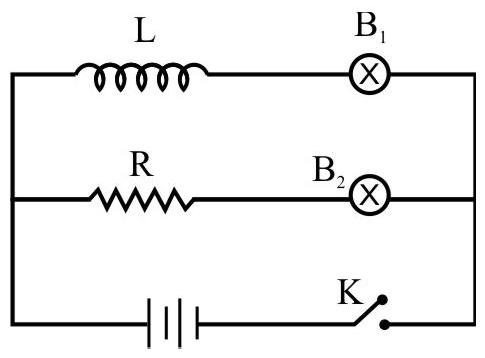
Experiment-2 :
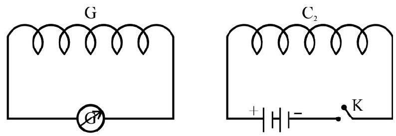
- It is observed that the galvanometer shows a deflection (momentary) when the current in
- When the key ’
- Similar effects are observed by increasing or decreasing the current in the coil
- It is also observed that the deflection increases, quite significantly, when an iron rod is inserted into the coils along their axis.
- Hence a changing current in one coil, is a source of induced current in another coil (neighbouring).
Faraday’s Law of Induction
Faraday stated these experimental observations in the form of a Law, called ‘Faraday’s Law of Electricmagnetic Induction’. The law is stated as follows:
“The magnitude of the induced emf, in a circuit, is equal to the time rate of change of the magnetic flx linked with the circuit.” Mathematically, the magnitude of induced emf is given by
For a closely wound coil of
where
The product
Lenz’s Law
The polarity, of the induced emf, is given by a rule, known as lenz’s law. The statement of the law is as follows:
“The polarity of induced emf is always such that it tends to produce a curernt, which opposes the change in the magnetic flux that induced it.
We can, therefore, combine Faraday’s Law and Lenz’s Law to write
The negative sign indicates the direction of the induced emf ’
It the circuit is closed, a current
Lenz’s law is in accordance with the principle of conservation of energy. It enables us to realize that it is the mechanical work, needed to be done to ‘move the magnet (towards the coil)’, that gets converted into the induced) eletrical energy.
Induced Current and Induced Charge
If, in a coil of
Here
The above equation shows that the total induced charge (that flows) does not depend upon the time interval ’
Example-1:
The magnetic flux, through a coil, present in a magnetic field, directed perpendicular to its plane, varies with time (in second) according to the relation.
Find the magnitude of the induced emf in the coil at
Show Answer
Solution :
We have
Also
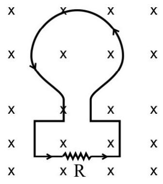
The direction of current, in the resistance
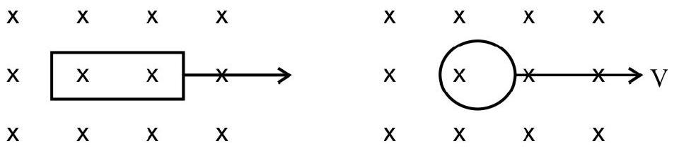
Example-2:
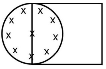
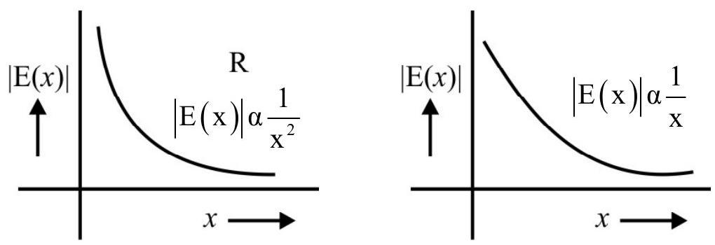
A rectangular loop, and a circular loop, are moving out of a uniform magnetic field region, to a field free region, with a constant velocity ’
Show Answer
Solution :
In case of circular loop, the rate of change of area of the loop, during its passage out of field region, is not constant. Hence induced emf will varry accordingly. In the case of the rectangular loop
Motion of a Conductor in a Uniform Magnetic Field
Let us consider a straight conductor, PQ, present in a, uniform and time independent magnetic field. As shown in the figure conductor ’
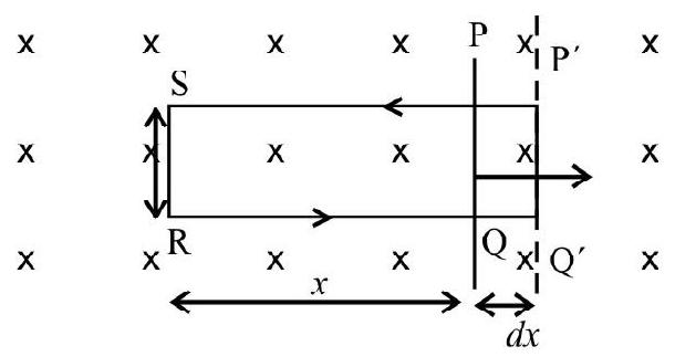
If the length
Since
But
Hence
The induced emf, BV
We can consider the above rod ’
Then, the induced current in the circuit will then be
From the above, we conclude that when a straight conductor, of length ’
Special Case :
If the direction of the velocity
Situation-1 :
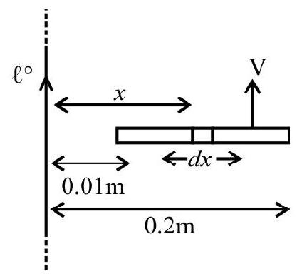
Consider a conducting rod
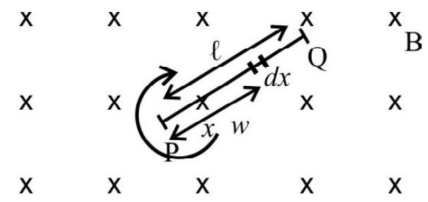
Consider a small element, of length
The induced emf ’
where
Thus,
If the rod moves about its centre, we would have
Energy Considerations : Let ’
On account of the presence of the magnetic field, there will be a lorentz force, on the arm ’
The magnitude of this force is
This force acts like a retarding force. Hence power is spend by an external agency to move the rod with a constant velocity ’
The power required to do this is given by
This power, spent by an external agent, is dissipated as Joule heat. The Joule heat produced is given by
Example-3:
A 10 meter long wire is kept in east west direction. It is falling down with a speed of
Show Answer
Solution :
(i) If a wire, of length
(ii) According to fleming left hand rule, the magnetic force on the electrons, in the wire, in the magnetic field will act towards west. Hence electrons will more to the western end of the wire, therefore the eastern end of the wire will be a higher (positive) potential.
Example-4:
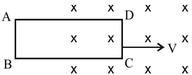
Ahorizontal metal frame,
Show Answer
Solution :
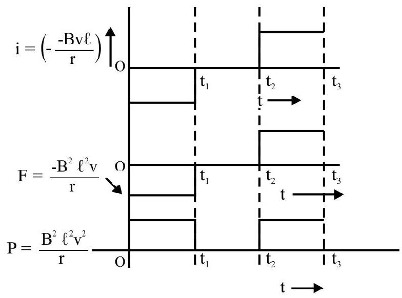
(i) The sides
(ii) As the whole frame in moving through the field from time
(iii) When
frame, is same, but its direction is now opposite to that in the first case (The flux is now decreasing with time). The required sketches, therefore, have the forms shown.
Example-5:
An air plane, with
Show Answer
Solution :
Here
We have
Example-6:
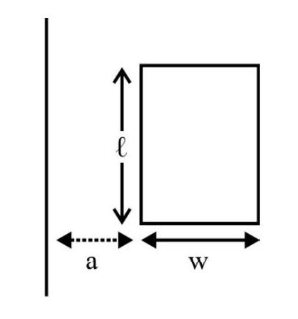
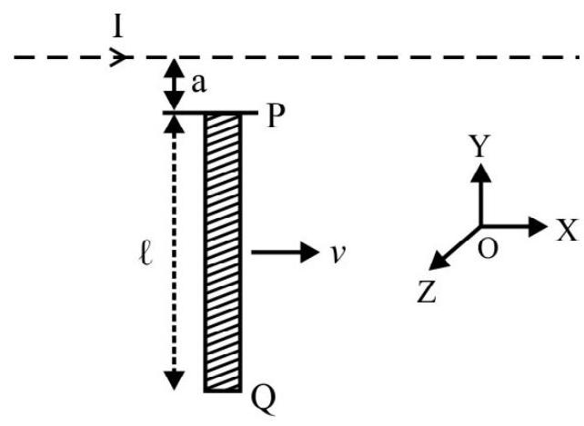
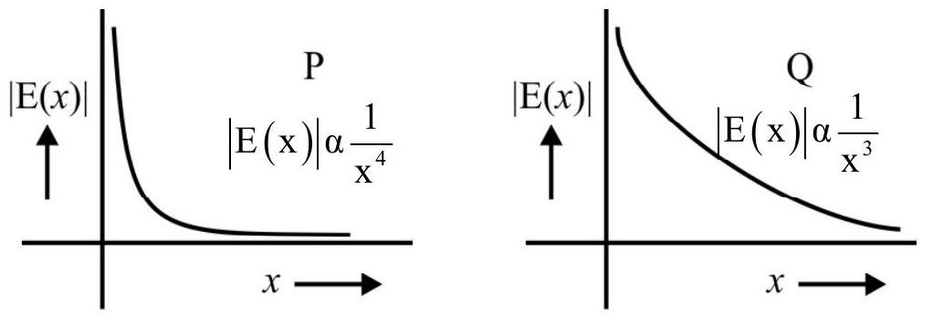
A copper rod, of length
Show Answer
Solution :
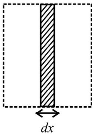
The magnetic field due to the long straight wire, at a distance ’
This field is directed into the page (downwards). If ’
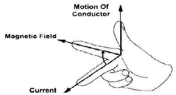
Flemings’s Right Hand Rule
The direction of the induced current, when a conductor moves in a uniform magnetic field, is given by Fleming’s right hand rule. This rule states that if we stretch the right hand thumb and the first two fingers, perpendicular to one another, and if the forefinger points in the direction of magnetic field, and the thumb in the direction of motion of conductor, the middle finger will point in the direction of the induced current.
Eddy Currents
Facoult, in 1895, discoverd that when a solid mass of metal is placed in a changing magnetic field, (or moved in a magnetic field), causing a change in the magnetic flux linked with it, induced currents are set up throughout the volume of the metal. These currents are known as ’eddy currents’ or ‘facault currents’. The direction of circulation of these currents is such as to oppose the motion of the metal or change in magnetic flux (in accordance with Lenz’s law).
The resistance of thick metal being very low, the eddy currents are generally quite large in magnitude and produce considerable heating effect in accordance with ‘Joule’s heating’ law. This heating effect of eddy
currents in undesirable in the interior of iron cores of rotating armatures of motors, dynamos and transformers etc. To minimize these currents, the cores are not taken as a single piece of soft iron but are made of many thin (insultated from each other) laminas of soft iron. This type of core is called a ’laminated core’.
Eddy currents are, however, also used to advantage in certain applications. These include:
(i) Electromagnetic Damping : Certain galvanometers have a fixed core made of a non magnetic metallic material. When the coil oscillates, the eddy currents, generated in the core opposes the motion and bring the coil to rest quickly.
(ii) Induction Furance : The metal to be heated, or melted, is placed in a high frequency changing magnetic field. Strong eddy currents, induced in it, cause heating.
(iii) Magnetic Brakes in Trains : Strong electromagnets are kept above the rails in some electrically powered trains. When the electromagnets are activated the eddy currents, induced in the rails, opposes the motion of the train.
Self Induction
We know that, when a current flows through a coil, it produces a magnetic field and hence a magnetic flux, which can be linked with the coil itself. It is possible that emf is induced in a single isolated coil due to change of flux through the coil itself by means of varying the current through the same coil. This phenomenon is called self-induction. The induced emf is called ‘back emf’.
Thus, when the current in a coil is switched on, the (induced) back emf opposes the growth of current. Similarly, when the current is switched off, the back emfopposes the decay of the current.
Let us consider a coil of
Here
When the current in the coil is varied, the flux linked with the coil also changes and an emf is induced in the coil. This is given by
The negative sign indicates that the selfinduced emf (or back emf) always opposes any change (increase or decrease) of current in the coil. From the above formula, we have
Hence the coefficient of self induction or self inductance of a coil is numerically also equal to the emf induced in coil when the rate of change of current, in the coil in unity.
The S.I unit of ’
We have
Also
Calculation of Self Inductance
It is possible to calculate the self in ductance for circuits with simple geometries.
Let us consider a long straight solenoid of cross section area
By definition, self inductance
Hence
If we fill the inside of the solenoid with a material of relative permability
Energy Associated with Self Inductance
Let
This work is stored in the form of magnetic potential energy
The above expression for the magnetic energy, stored in the magnetic field of solenoid, can be rewritten as
This expression is similar to electrostatic potential energy stored per unit volume in the electric field. In both cases energy is propotional to the square of the (corresponding) field strength.
An ideal solenoid, or coil, whose inductance
We have derived the formula for energy density, for the special case of the uniform magnetic field of an ideal solenoid (inductor), the result is a geenral one and is valid for any region of space in which a magnetic field exists.
Mutual Induction
Let there be two coils in close proximity of each other. When the current in one of these coils changes, the magnetic field due to it over the other coil changes. Hence the magnetic flux linked with the other coil also changes and an emf is induced in this neighbouring coil. Such a phenomenon is known as mutual induction. The (first) coil, in which the current changes (leading to change in magnetic flux linked with the second coil), is called the primary coil. The second coil, in which induction takes place, is called the secondary coil.
Let
or
where
’
Hence mutual inductance, for a pair of coil, is equal to the induced emf, set up in one coil due to unit rate of change of current in the other coil.
The SI Unit of
The value of mutual inductance of a given pair of coils, depends upon the number of turns of the coils their geometrical shape and size, their relative separation as well as their relative orientation. It also depends upon the permiability of the medium in the space between the two coils.
Consider two long co-axial solenoids each of length ’
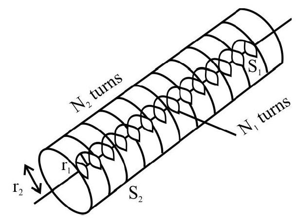
When a current
Also
This implies that
If we consider the reverse case, the flux linkage, due to current
This implies that
We thus see that
Hence, in general one can write that, for a pair of solenoidal coils
Here
Special Case-I :
Consider the general case of currents flowing simultaneously in two nearby coils. The flux linked with one coil will be the sum of two fluxes which exist independently. We can write
Here
Hence the total induced emf, in coil ’
Special Case-II :
(a) When two ideal solenoids (inductors), of self inductances
If flux, of one coil, favours the other, then
and if flux, of one coil, opposes the other, then
(b) If the coils are seperated by a large distances,
(c) If two inductor are connected in parallel, turns out that
For isolated coils (or for large separation of two coils)
(d) The coefficient of coupling,
Example-7:
A small circular loop, of radius
Show Answer
Solution :
By symmetry, the flux linked with the bigger loop, due to current in the smaller loop, will be same as the flux linked with the smaller loop, due to the same current in the bigger loop (
Now the magnetic field, at the centre of smaller loop, due the to a current, i, in the bigger loop, is
The field
This is the same as the flux
Example-8:
A very small circular loop of area
Show Answer
Solution :
The magnetic field, at the centre of larger loop, is
Magnetic flux, linked with the smaller loop (of area
The induced emf, in the smaller
Induced emf in a planer coil,due to a change in its orientation in a uniform magnetic field
Let a planer coil, having
From Faraday’s law, induced emf in the rotating coil, is
This is the instantaneous value of induced emf. Clearly
Hence induced emf, in the coil, varies with time in a sinusoidal way. When the plane of the coil is parallel to B
This method, of producing a flux change, due to a change in the loop’s orientation,
An a.c. generator converts mechanical energy into electrical energy. In commercial generators, the mechanical energy, required for rotation of the coil, is provided either by water falling from heights in dams (hydroelectric generators) or by steam at high pressure, produced in thermal generators. Nuclear energy is now also being increasingly used, for this purpose, in the so called nuclear energy powered electric generators.
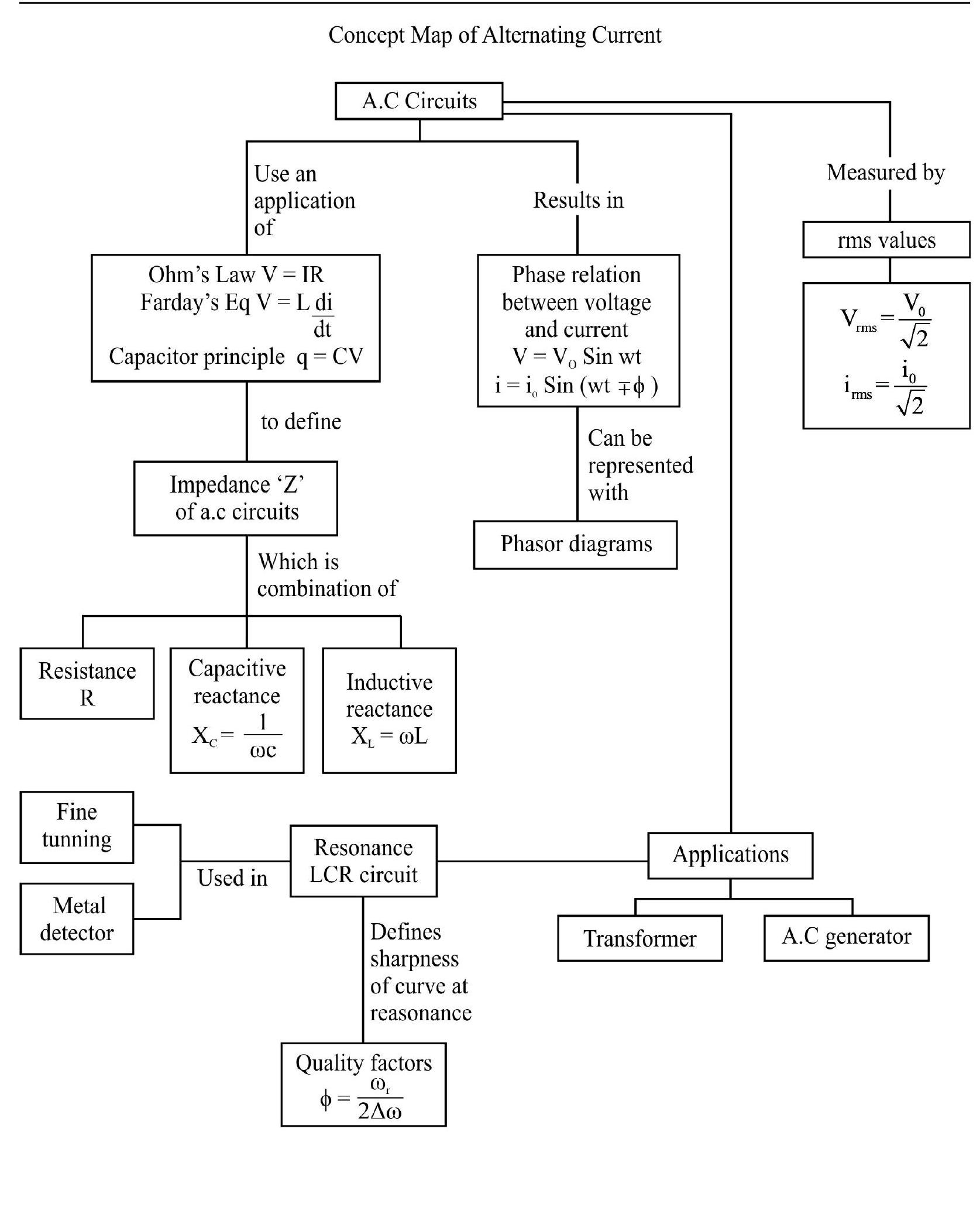
Alternating Current
Alternating current is that current which continuously varies in magnitude and periodically reverse its direction. The same is true for alternating emf’s or voltages.
The simples type of alternating current is one which varies with time is a simple harmonic (sinusoidal) way. It is represented by
where is the instantaneous value of curernt, at time
Here
Mean (or Average) Value of A.C.
An alternating current (or voltage) flows, during one half cycle, in one direction, and during the other half cycle in opposite direction. Hence for one complete cycle the mean value of the a.c. would be zero. This is why there is no (net) deflection in a moving coil galvanometer when an alternating current passes through it. Average value over full cycle
However, the mean value, of a sinusoidal a.c, over a half cycle, has a finite value.
Mean, or average value over half a cycle, is given by
We thus notice that the mean value, of a simusoidal a.c., over a half cycle, is
Root mean Square Value of a.c
The root mean square (r.m.s) value of a.c is defined as the square root of the average value of
Now, average value of
This comes out to be
Hence, the root mean square value of a sinosoidal a.c, is given by
Thus, the root mean square value of an a.c, is
In a similar way,
Physical Significance of r.m.s Value
If an a.c,
The ‘average’ rate of production of heat, over one complete cycle of current, is then given by
Now if one passes a direct current, of strength
Hence, the root mean square value, of an a.c., is also called as the ’effective value’ or the ‘virtual value’ of the given a.c. The measurable value of an a.c. is thus its r.m.s value, or ’effective (or virtual) value’. The ammeter or voltmeter designed to measure a.c., would directly give the relevant r.m.s value. In our houses, alternating current is supplied at
‘Phasors’ or Phasor Diagrams
In an a.c. circuit, the frequency of the alternating current and alternating emf is same. However, it is not necessary that they both be in the same phase. Usually, when the current in the circuit in maximum, the emf is not maximum and vice-versa. The phase difference between the two, depends upon the type of circuit. Phase of a.c may be defined as the time period that has elapsed. Since the current (or emf) last passed its zero value in the positive direction.
The study of a.c circuits is much simplified if we treat alternative current or alternating emf as (kind of) vectors. The angle between the ‘vectors’ representing current and voltage is taken equal to the phase difference between them. The current and emf ‘vectors’ are better called ‘phasors’. Adiagram, representing alternating current and emf as ‘phasors’, showing the phase angle between them, is called a ‘Phasor Diagram’.
AC Voltage applied to a Resistor
Let an alternating voltage
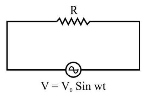
Hence
where
The above expression shows that in a pure resistance, the current is always in phase with the applied voltage.
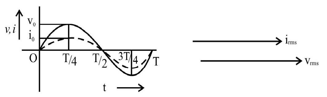
The above graphical representation shows this. It shows that both
The average value of
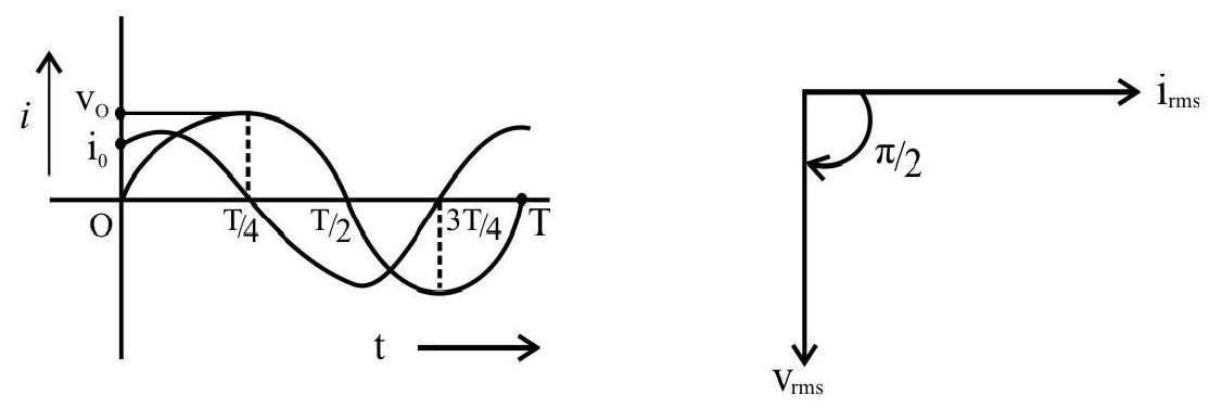
AC Voltage applied to a Pure Inductor
Let an alternating voltage,
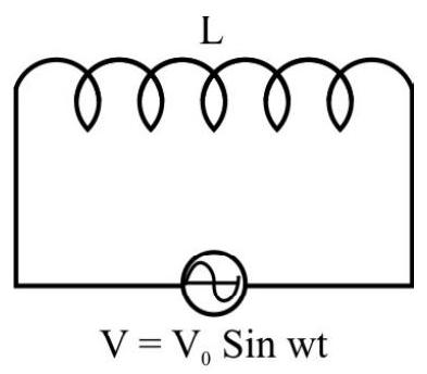
On integrating both sides, we get an expression for the instantaneous current in the circuit. We have
or
or
Here
A comparison of this equation with the voltage equation, shows that, in a pure inductor, the current lags behind the applied voltage by a phase angle of
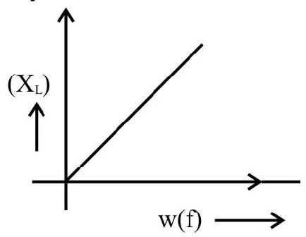
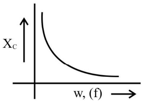
As
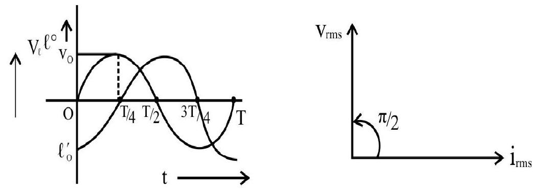
The inductive reactance increases with frequency, in a linear, or proportinoal way.
We can also write,
The instantaneous power supplied to the inductor is
The average power, over a complete cycle, is given by
This comes out to be zero i.e.
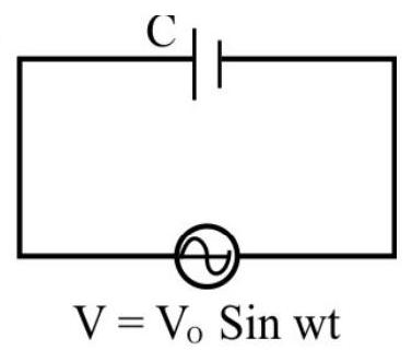
AC Voltage applied to a Pure Capacitor
Let alternating voltage,
Let
The instaneous current in the circuits is, therefore, given by
or
where
A comparison of this equation with the voltage equation shows that, in a pure capacitor, current is ahead of voltage by a phase angle of
As
Thus capacitive reactance decreases with increase in freqeuncy. As
We can also write,
The instantaneous power supplied to the capacitor is
The average power, over a complete cycle,
This comes out to be zero.
This means that energy is absorbed from the source during one quater cycle (when capacitor is getting charged). In the next quater cycle, energy gets returned to the source, (as capacitor gets discharged over a complete cycle), the capacitor thus acts like a ‘wattless’ element.
To summarise:
| Pure R | Pure L | Pure C |
|---|---|---|
| v lags behind i (in phase) by |
AC Voltage applied to Inductor and Resistor in Series (LR Series Circuit)
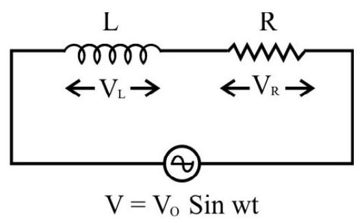
Let an alternating voltage,
or
The term
Thus, here
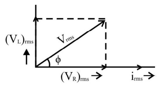
Also,
The phasor diagram shows that, in a series LR circuit, the voltage (still) leads the current, now by a phase angle
The inductive effect dominates in a series LR circuit. This means that the voltage reaches its maximum value
Example-9:
A students connects a long air cored coil, of manganin wire, to a
Show Answer
Solution :
In d.c circuit the impedance of the coil, is only due to its resistance ’
When the same coil is connected to an a.c source, the impedance of the coil is due to both its resistance
The value of current, in the a.c circuit decreases, because of this increase in impedance of the coil.
Now
Example-10:
An inductor ’
Show Answer
Solution :
We have
Hence algebric sum of p.d. across
AC Voltage applied to a Capacitor and a Resistor in Series (RC Series Circuit)
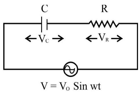
Let an alternating voltage,
Thus,
or
Here
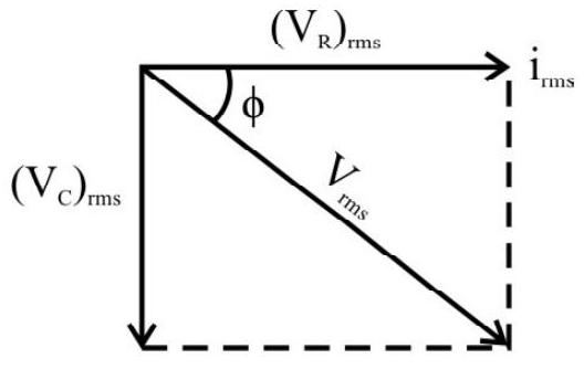
It is called the impedance of this circuit and is denoted by
and
The phasor diagram shows that in the
The capacitive effect dominates in this circuit. This means that the current reaches its maximum value
Example-11:
A
Show Answer
Solution :
Time lag
Here
Now
AC Voltage applied to a Pure Inductor and a Pure Capacitor in Series (LC Series Circuit)
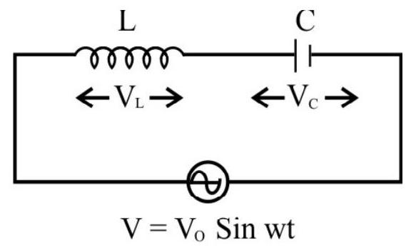
In this case, voltage across
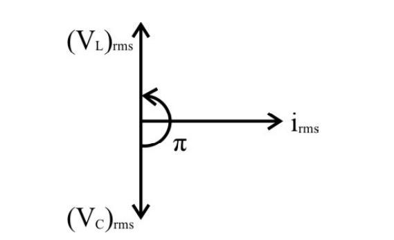
Hence
Here
Special Case:
(i) If, in this circuit,
When
or
This frequency value (
(ii) If
(iii) If
AC Voltage applied to Series LCR Circuit
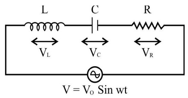
Let an alternating voltage,
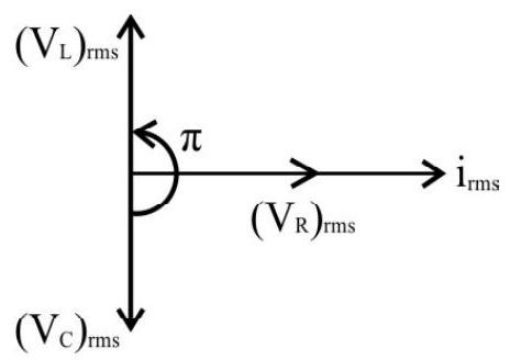
Case (i) :
If
We, therefore, have
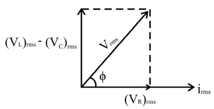
Here, the impedance of the circuit, ’
Here
Hence the inductive effect dominates in such a circuit. The applied voltage,
This means that the voltage reaches its maximum value
Case (ii) :
If
We, therefore, have
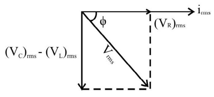
Here the impedance of the circuit, ’
Here
or
This means that voltage reaches its maximum value
The instantaneous current
Case (iii) :
An interesting characteristics of the series LCR circuit is the phenomenon of resonance.
For an LCR circuit, driven with applied voltage of amplitude
Here
The impedance of the circuit is then at its minimum value
At resonant frequency the current amplitude is maximum
For values of
Resonant circuits have a variety of applications. These include, among others, the tunning circuits of a radio or T.V. set, and the working of metal detectors.
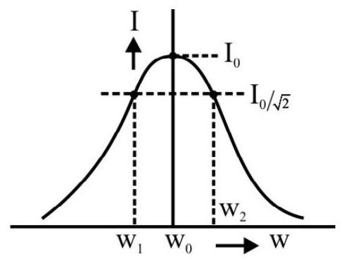
Sharpness of Resonance
Suppose we choose a value of
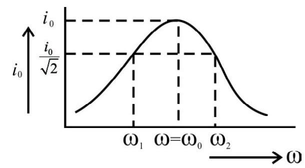
From the graph between
The difference,
The sharpness of resonance is, therefore, given by
The ratio
Example-12:
An a.c. source of frequency
Show Answer
Solution :
Here inductive reactance
Capacitive reactance
Thus
Example-13:
AnLCR series circuit, with resistance
Show Answer
Solution :
We have
or
This implies that circuit is at resonance.
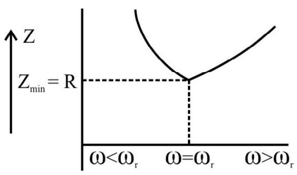
Example-14:
Sketch the variation of impedance (z) with angular frequency
Show Answer
Solution :
We have
At
Further,
For
Power in a Series LCR AC Circuit
When a voltage,
[negative sign for inductive effect and positive sign for capacitive effect]
Therefore, the instantneous power ’
The average power over a full cycle is given by
\
This can be written as
So, the average power dissipated in the circuit depends not only on the rms values of voltage and current
but also on the phase angle,
The quantity ’
Case (i)
Resistive Circuit : If the circuit contains only a pure resistor, there voltage and current are in same phase i.e.
Case (ii)
Purely inductive or capacitive or a series LC circuit: If the circuit contains only a pure reactance ’
Case (iii)
LCR Circuit : In a series LR, RC or a series LCR circuit,
Case (iv)
LCR circuit at resonance : At resonance
Example-15:
A series LR circuit draws a power of
Show Answer
Solution :
We are given that
Power dissipated
This gives
and
The power factor would become unity if a capacitor,
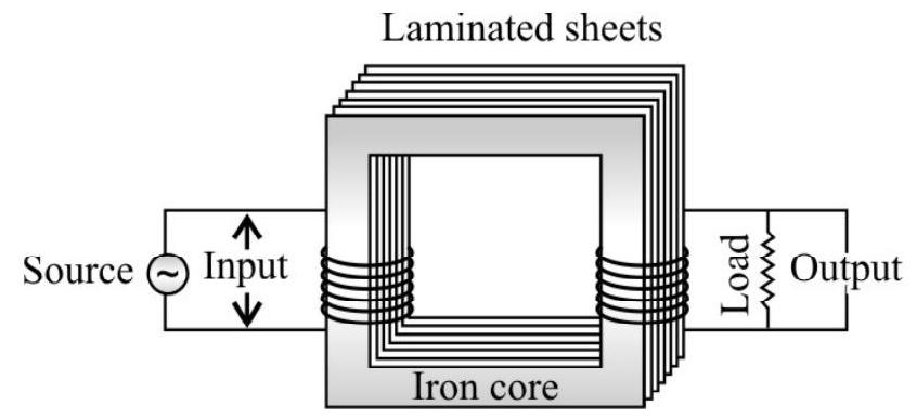
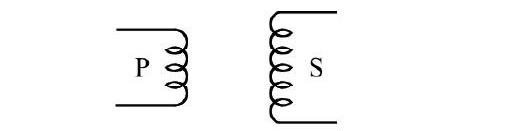
Transformer
It consists of two coils wound on the same core. The alternating current passing through the primary creates a continuously changing flux through the core. This changing flux induces an alternating emf in the secondary.
(1) Transofrmer works on ac only and never on d.c.
(2) It can increase or decrease either voltage or current but not both simultaneously.
(3) Transformer does not change the frequency of input a.c.
(4) There is no electrical connection between the winding but they are linked magnetically.
(5) Effective resistance between primary and secondary winking is infinite.
(6) The flux per turn of each coil must be same i.e.
(7) If
As in an ideal transformer there is no loss of power i.e.
Types of Transformer
| Step up transformer | Step down transformer |
|---|---|
| It increases voltage and decreases current | It decreases voltage and increases current |
 |
 |
Efficiency of transformer (h): Efficiency is defined as the ratio of output power to input power i.e.
For an ideal transformer
For practical transformer
so
(9) Losses in transformer : In transformers some power is always lost due to, heating effect, magnetic flux leakage, eddy currents, hystersis and humming.
(i)
(ii) Eddy Current loss : Some electrical power is wasted in the form of heat due to eddy currents induced in core, to minimize this loss transformers core are laminated and silicon is used as the core material as it increases the resistivity. The material of the core is then called alloy of iron (steel).
(iii) Hystersis loss: The alternating current flowing through the coils magnetises and demagneties the iron core again and again. Therefore, during each cycle of magnetisation, some energy is lost due to hysteresis. However, the loss of energy can be minimised by selecting the suitable of core, which has a narrow hysterisis loop. Therefore core of transformer is of soft iron. Now a days it is made of “Permalloy”
(iv) Magnetic flux Leakage : Magnetic flux product in the primary winding is not completely linked with secondary becuase few magnetic field lines complete their path in air. To minimize this loss secondary winding is kept inside the primary winding.
(v) Humming losses : Due to the passage of alternating current, the core of the transformer starts vibrating and produces humming sound. Thus, some part (may be very small fraction) electircal energy is wasted in the form of humming sound produced by the vibrating core of the transformer.
(10) Uses of transformer : A transformer is used in almost all a.c. operation e.g.
(i) In voltage regulators for TV, refregerator, computer, air conditioner etc.
(ii) In the induction furnances.
(iii) Step down transformer is used for welding purposes.
(iv) In the transmission of a.c. over long distance.
PROBLEMS FOR PRACTICE
1. A long solenoid of radius
Show Answer
Answer:2. A coil of area
Show Answer
Answer: (i)3. In an aeroplane, the distnace between the edges of its wings being
Show Answer
Answer: (i)4. A conducting loop of area
Find (a) the maximum emf induced in the coil (b) the emf induced at
Show Answer
Answer: (a)5. An air cored coil has a self inductance of
Show Answer
Answer:6. In the given circuit, the resistance ’
7. A conducting circular loop of area
Show Answer
Answer:8. A uniform magnetic field
Show Answer
Answer:9. Figure shows a bar magnet
10. Two coils
Show Answer
Answer:11. An alternating voltage
Show Answer
Answer: (i)12. When and inductor
Show Answer
Answer:13. An alternating emf
14. The voltage
Dtermine the phase difference between
Show Answer
Answer:15. In the given LCR series circuit fed by
Show Answer
Answer: (i)16. A
Show Answer
Answer:17. A current of
Show Answer
Answer:18. An
Show Answer
Answer:19. A step down transformer having a power output of
Show Answer
Answer: 5000, 1.01 A20. An a.c. source of internal resistance
[Hint:
Show Answer
Answer: 30Question Bank
Key Learning Points
1. The magnetic flux through a surface of area
where
2. The emf, induced in a coil of
where
3. When a metal rod of length
4. For a rod rotating about its one end, in a uniform magnetic filed, about an axis perpendicular to the rod, with the magnetic field parallel to the axis, the emf induced between its two ends,
5. Changing magnetic fields can set up current loops in nearby metal bodies. They dissipate electrical energy as heat. Such currens are called eddy currents.
6. When a current in a coil changes, it induces back emf in the same coil. The self induced emf is given by
where
7. The self inductance (or inductancee) of a long (ideal) solenoid (the core of which has a permability) is given by
8. A changing current, in one coil, can induce an emf in another (nearly) coil. The emf induced, in the second coil, in given by
For two coaxial (long) solenoids placed such that one is completely placed well inside the other, the mutual inductance is given by
where
9. When a coil, of
Here,
10. The mean, or average, value ofan alternating voltage (or current) over a complete cycle is zero. Over a half cycle, the mean value is
11. The r.m.s value of current is given by
Similarly
12. An alternating voltage
13. An a.c voltage,
14. An a.c voltage,
15. In a series LCR circuit, if a voltage
Case (i):
or
Inductive effect dominates in the circuit. Voltage leads the current by phase angle
Case (ii):
or
Capacitive effect dominates in the circuit. Current leads the voltage by phase angle
16. An interesting characterstics of a series LCR circuit is the phenomenon of resonance.
17. The quality factor,
’
18. The average power dissipation, or loss of power over a complete cycle, is given by
The term,
19. In pure inductive, or capacitive or a series (LC) circuit, the power factor,
20. A transformer consists of an iron core on which are bound a primary coil of
The currents are related by
In step up transformer
and in step down transformer
Easy
Self Induction
1. When the current in a coil changes from
(1)
(2)
(3)
(4)
Show Answer
Correct answer: (1)
Solution:
Average
Induced emf
2. A conducting circular loop is placed in a uniform magnetic field
(1)
(2)
(3)
(4)
Show Answer
Correct answer: (2)
Solution:
Difficult
Change in Magnetic Flux
3. A magnetic field, directed along
(1)
(2)
(3)
(4)
Show Answer
Correct answer: (2)
Solution:
We have,
Initial total flux
In one second the loop covers a distance of
This flux comes out to be
Difficult
Induced emf
4. A conducting ring, of radius
(1)
(2)
(4)
Show Answer
Correct answer: (2)
Solution:
Let
From (1) and (2)
Difficult
Power Loss
5. Magnetic flux, through a stationary loop, with a resistance
(1)
(2)
(3)
(4)
Show Answer
Correct answer: (3)
Solution:
We have,
Instantaneous power loss / dissipation
Average
Self Induction
6. The current, through a coil of self inductance.
(1)
(2)
(3)
(4)
Show Answer
Correct answer: (2)
Solution:
We want to have
Difficult
Induced emf
7. The magnetic flux
(1)
(2)
(3)
(4)
Show Answer
Correct answer: (1)
Solution:
We have
Average
LC Oscillations
8. An LC circuit contains a
(1)
(2)
(3)
(4)
Show Answer
Correct answer: (2)
Solution:
Total energy, in a LC circuit, is completely magnetic (at first) at
Here
Easy
Induced emf due to Change in Orientation
9. A rectangular coil, of 300 turns, has an average area of
(1)
(2)
(3)
(4)
Show Answer
Correct answer: (2)
Solution:
Easy
Change in Magnetic Flux / Lenz’s Law
10. Two identical coaxial coils,
(1)
(2)
(3) both P and Q increases
(4) both P and Q decreases
Show Answer
Correct answer: (4)
Solution:
When both the coils are brought closer. The linked magnetic flux, increases for both of then. Hence induced current (set up in then) will try to decreases the flux (as per Lenz’s law). Hence current in both the coils will decrease.
Easy
Induced emf
11. A 50 turns circular coil has as average a radius of
(1)
(2)
(3)
(4)
Show Answer
Correct answer: (3)
Solution:
Change in magnetic flux, linking the coil, is
Average
Induced emf
12. A conducting circular loop is placed in a uniform magnetic filed (of induction ’
(1)
(2)
(3)
(4)
Show Answer
Correct answer: (2)
Solution:
The magnetic flux, linking the loop, (when its radius is
Average
Motion of a Conductor in Magnetic Field
13. A conducting rod of length
(1)
(2)
(3)
(4)
Show Answer
Correct answer: (2)
Solution:
The induced emf, across a small element dy of the rod is
Average
Induced emf and Current
14. The magnetic flux, through a circular coil of resistance
(1)
(2)
(3)
(4)
Show Answer
Correct answer: (4)
Solution:
The induced emf in the coil will be given by
Average
Induced Current
15. A cylindrical bar magnet is rotated about its axis as shown in the diagram. One end of a wire is connected to apoint on the axis and its other end is made to touch the cylindrical surface through an ammeter. We would then observe
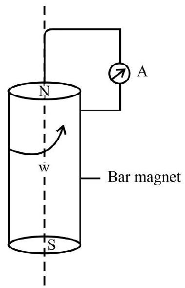
(1) That a direct current flowing in the ammeter
(2) That no current flows through the ammeter A
(3) That an alternating simusoidal current flows through the ammeter A
(4) Atime varying, non-simusoidal, current flows through the ammeter A
Show Answer
Correct answer: (2)
Solution:
As there is no change in the magnetic flux linked with the circuit, no emf gets induced in the circuit. The ammeter ’
Average
Induced emf and Current
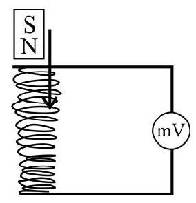
16. A magnet NS is suspended from a spring. While it oscillates simple harmonically, it moves in and out a coil ’
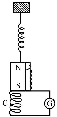
As the magnet oscillates (Simple harmonically)
(1) G shows no deflection at all
(2) G shows deflection, alternately, to the left and right, but its amplitude keeps on changing
(3) G shows deflection, alternately, to the left and right, with a constant amplitude
(4) G shows a deflection on one side only
Show Answer
Correct answer: (2)
Solution:
As the magnet moves in and out of the coil, there is a continuous change in the magnetic flux linked with the coil. The flux first increases (as magnet moves in) and then decreases (as magnet moves out). Hence the induced emf keeps on changing.
The motion of the magnet is S.H.M. (an accelerated motion). Hence
Difficult
Magnetic Flux
17. A loop, made of straight edges has six corners: at
(1)
(2)
(3)
(4)
Show Answer
Correct answer: (2)
Solution:
Given
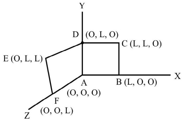
The area vector of part
and that of part DEFA is
Total flux linking to the loop will be
Average
Induced emf
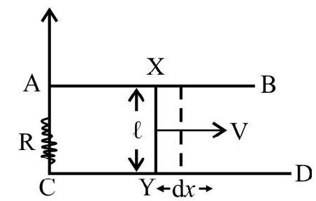
18. A conducting wire
(1)
(2)
(3)
(4)
Show Answer
Correct answer: (3)
Solution:
Let, at time
The magnetic flux associated with the area ACYXA, (at time t) will be
This magnetic flux changes with time due to two reasons. There are:
(i) The change of the magnetic field itself with time.
(ii) The motion of the wire on the rods.
We can, therefore, write
The force, on wire
From (1) & (2), we get
Average
Motion of a Conductor in Uniform Magnetic Field
19. In a uniform magnetic field of induction
(1)
(2)
(3)
(4)
Show Answer
Correct answer: (2)
Solution:
We have
The average value of
Average
Motion of a Conductor in Uniform Magnetic Field
20. A straight rod
(1)
(2)
(3)
(4)
Show Answer
Correct answer: (1)
Solution:
The potential difference, between two ends of a rod, confined at one end, is given by
(
and
Difficult
Induced emf
21. A thin semicircular conducting ring, of radius

(1)
(2)
(3)
(4)
Show Answer
Correct answer: (3)
Solution:
Rate of decrease of area, of the semicircular ring, in the magnetic field, for the position MNQ, will be
Now
As per Lenz’s law, the induced current in the ring must produce magnetic field directed ‘outwards’. Thus Q must be at a higher potential (so as to send the required anticlockwise (induced) current in the ring).
Easy
Self Induction
22. A conducting coil of 600 turns has a self inductance of
(1)
(2)
(3)
(4)
Show Answer
Correct answer: (1)
Solution:
We know that
Average
Self Induction
23. The current ’ 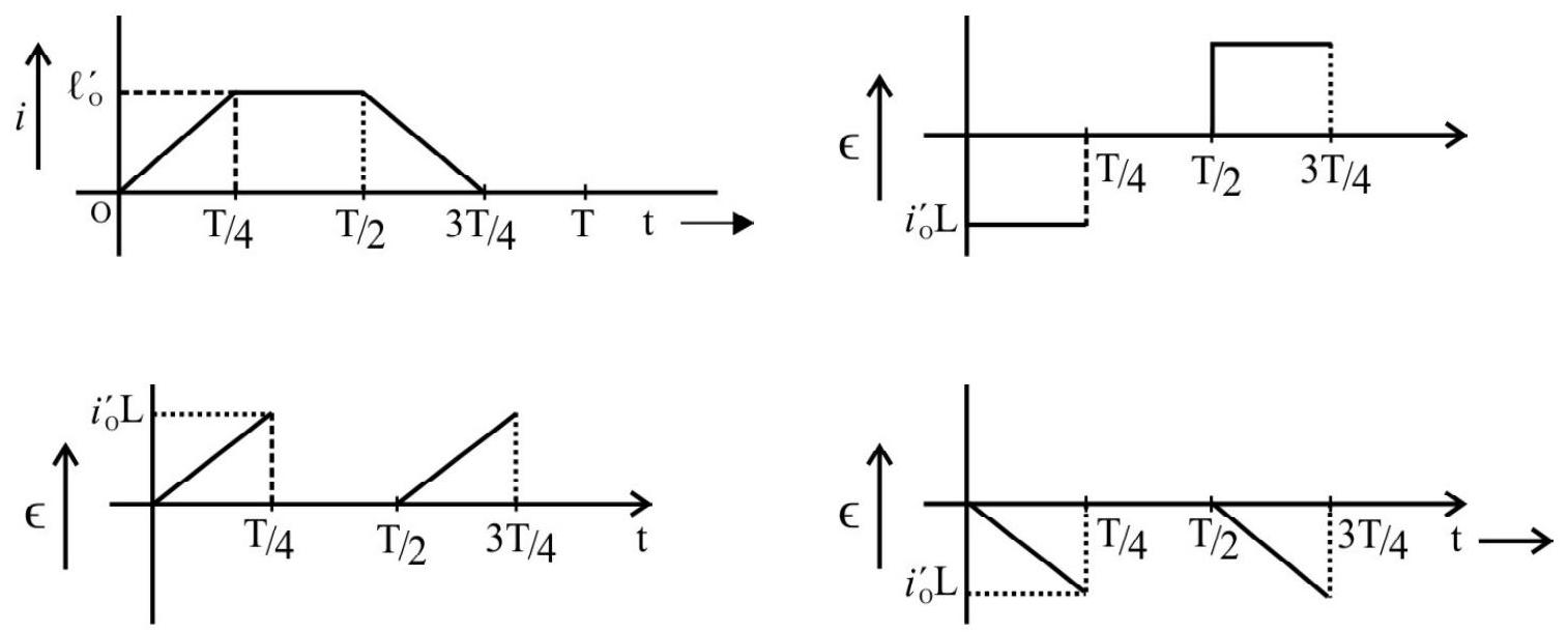
(1)
(2)
(3)
(4)
Show Answer
Correct answer: (1)
Solution:
We have
During 0 to
For time
For time
Hence
Average
Self Induction
24. A (solenoid) coil is wound on a core of square cross-section. If all the linear dimensions of core are increased 2 times, but the number of turns per unit length of the coil, remains same, the self inductance would increases by a factor of
(1) 2
(2) 4
(3) 8
(4) 16
Show Answer
Solution:
The self inductance of the coil is given by
For a square core
The self inductance, therefore, increases by a factor of 8 .
Average
Mutual Induction
25. A pair of (insulated) coils having of
(1)
(2)
(3)
(4)
Show Answer
Correct answer: (4)
Solution:
Induced emf, due to mutual induction between in two coils, is given by
We are given that
We know that
Average
Mutual Induction
26. The coefficient of mutual inductance of two circuits
(1)
(2)
(3)
(4)
Show Answer
Correct answer: (1)
Solution:
We have
Average
Mutual Induction
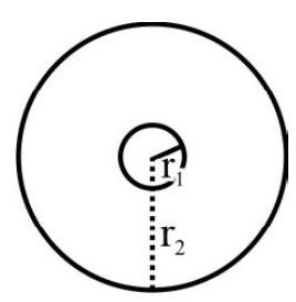
27. Consider two coplanar, co-centric circular coils having radii
(1)
(2)
(3)
(4)
Show Answer
Correct answer: (1)
Solution:
We will consider the bigger coil as the primary coil. In the expression
we put the value of
Difficult
Mutual Induction
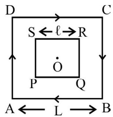
28. A small square loop of wire, of side
(1)
(1)
(2)
(3)
(4)
Show Answer
Correct answer: (2)
Solution:
The bigger loop may be taken as primary coil and the smaller one as the secondary coil. (We need to use the expressions for the magnetic field due to a finite wire). The bigger coil can be considered as equivalent to four current carrying long wires. All these wires, it can be seen produce magnetic fields in the same sense. Hence net magnetic field at the centre, will be
The flux, linked with the smaller loop, will be
Also
We can assume the magnetic field to
or
From (1) & (2), we get
Easy
Self + Mutual Induction
29. Two (insulated) coils are wound, (one over the other), on a solenoid core. If the number of turns, per unit length, of the first ciol and of the second coil, were to be increased by a factors of 3 and 4 , respectively, the self inductance of the two coils
(1) 3,4 and 12
(2) 3, 4 and
(3) 9,16 and
(4) 9,16 and 12
Show Answer
Correct answer: (4)
Solution:
We know that the self inductance, of a solenoidal coil, is proportional to
Hence the self inductances, of the two coils will increase by factors of
]
The mutual inductance of the two solenoid coils (one over the other) is proportional to the product
Hence M, in the given case, would increase by a factor of
Average
Energy Associated with an Inductor
30. A spring, of spring constant
The self inductance of the coil equals
(1)
(2)
(3)
(4)
Show Answer
Correct answer: (2)
Solution:
The P.E., of a compressed spring
The work, needed to be done, to establish a current I, in a coil of self inductance L, equals
We, therefore, have
Average
Induced emf
31. A circular ciol, of average radius
A small rectangular lamina of sides
(1) zero
(2)
(3)
(4)
Show Answer
Correct answer: (3)
Solution:
The magnetic field, due to the current carrying circular coil, at the centre of the rectangular lamina
The field can be assumed to have this (nearly) constant magnitude all over the plane of the small lamina. Hence the change in flux through it, when it is ‘flipped over’ is
Average
Induced Current
32. A rod,
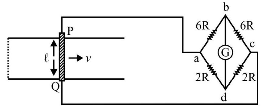
(1)
(2)
(3)
(4)
Show Answer
Correct answer: (1)
Solution:
The emf, induced in the rod, equal
The wheatstone bridge, abcd, as shown is a balanced bridge. Its equivalent resistance,
This gives
The total resistance of the circuit is, therefore
In the wheatstone bridge, the part,
Hence
This given
Average
Force due to Induced Current
33. The set-up, shown in the figure, is present in a uniform magnetic field,
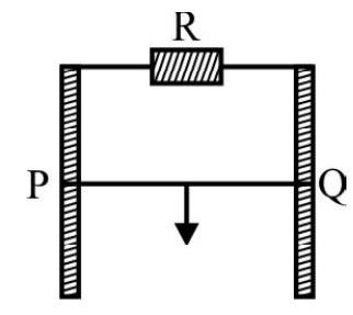
(1)
(2)
(3)
(4)
Show Answer
Correct answer: (4)
Solution:
As the rod PQ slides down, the magnitude of the induced emf, in it, at an instant when its velocity is v, equals
Average
Induced Charge Flow
34. A small coil, having
The graph that best shows the dependence of the charge flowing
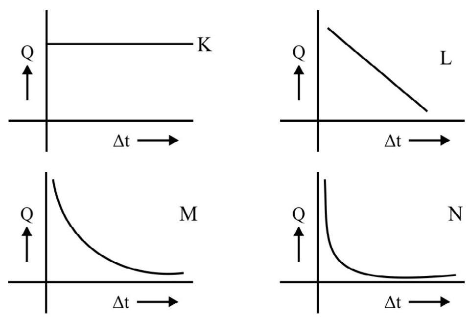
(1)
(2)
(3)
(4)
Show Answer
Correct answer: (1)
Solution:
Let
The linked magnetic flux becomes zero when it is withdrawn from the field. The instantaneous induced emf, would be
The instantaneous induced current
Average
Self Inductance of a Solenoid
35. A solenoid, having a total of
(1)
(2)
(3)
(4)
Show Answer
Correct answer: (2)
Solution:
The magnetic field, B, along the axis of this (long) solenoid, equals
The flux,
We also have
We thus get
Average
Slef + Mutual Inductance
36. A (long thin) solenoid core has an insulated primary coil, (of
If
(1)
(2)
(3)
(4)
Show Answer
Correct answer: (2)
Solution:
The self inductance,
and
when
We, therefore, have
[Alternatively: We know that, in the dieal case, the coefficient of coupling between the two coils, equals unity.
Now
Average
Mutual Inductance of a Pair of Coils
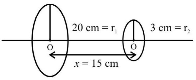
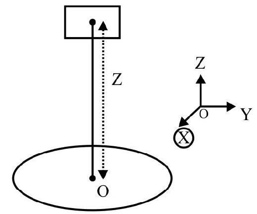
37. Two circular loops, of radii
(1)
(2)
(3)
(4)
Show Answer
Correct answer: (4)
Solution:
We imagine a current I to flow through the larger loop. The magnetic field, due to it, at the centre of the small loop, would then equal
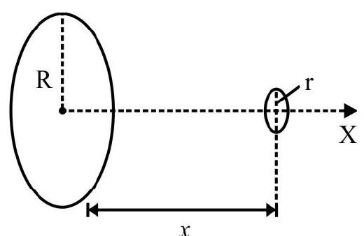
The small coil has a very small radius. We may, therefore, assume that the magnetic flux, linked with it, is (nearly)
But
Hence
For
Difficult
Mutual Inductance
38. A long straight wire and a planer rectangular loop are present in the vicinity of each other in the
(1)
(2)
(3)
(4)
Show Answer
Correct answer: (3)
Solution:
We imagine a current I to flow through the long straight wire. The magnetic field, due to it at any point (in the xy plane), distant
The total magnetic flux, linked with the rectangular loop, is
But
Hence
Difficult
Motional emf
39. A (infinite) long straight wire, carrying a current
(1) zero
(2)
(3)
(4)
Show Answer
Correct answer: (3)
Solution:
The magnetic field, due to the long straight current carrying wire, would have different magnitudes on the different elements of the straight conductor PQ. However its direction, at all these elements, is directed along
Difficult
Induced emf
40. A circular coil, of radius
A small rectangular lamina, of area
(1)
(2)
(3)
(4)
Show Answer
Correct answer: (1)
Solution:
The set-up, of the ‘system’, is as shown here.
The magnetic field, due to the current carrying circular coil, at the centre of the rectangular lamina (when this centre is at a distance
The rectangular lamina, being a small sized one, the magnetic flux, linked with it, can be written as
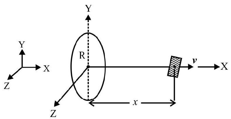
We are given that
The instantaneous induced emf,
Difficult
Power Factor and Quality Factor in a Series LCR Circuit
41. A voltage source,
(1)
(2)
(3)
(4)
Show Answer
Correct answer: (2)
Solution:
The phase angle, Q, (current lagging), between the current flowing and the applied voltage, in a series LCR circuit, is given by
In the given case,
The quality factor,
Average
Voltage Magnification in a Series LCR Circuit
42. A series LCR circuit can bring about a ‘voltage magnification’, of the voltage of the a.c. source connected across it, provided the frequency, of the a.c. voltage source, equals
(1)
(2)
(3)
(4)
Show Answer
Correct answer: (3)
Solution:
The resonant frequency, for the series LCR circuit, equals
For a voltage source, having this frequency, the net impedance of the circuit equals R. Hence the source voltage equals the voltage drop
The total voltage drop, across the combination of
At the resonant frequency, voltage drop across
Easy
Sharpness of Resonance
43. In A.C.voltage source,
(1)
(2)
(3) (nearly)
(4) (nearly)
Show Answer
Correct answer: (2)
Solution:
The current value, for
Further, the more the value of
Difficult
Power Factor and Quality Factor of a Series LCR Circuit
44. A voltage source,
(1)
(2)
(3)
(4)
Show Answer
Correct answer: (1)
Solution:
The power factor, of a series LCR circuit, equals
For the given circuit :
Hence
Also
Here
Average
Q-Factor
45. For a given series LCR circuit, the term
(1) is a dimensionless term that provides a measure of (i) the quality factor (Q) and (ii) the power factor of the circuit at resonance
(2) is a dimensionless term that provides a measure of (i) the sharpness of resonance (S) and (ii) the voltage magnification of the circuit at resonance
(3) is a dimensional term that provides a measure of the (i) voltage magnification of the circuit at resonance and (ii) the sharpness of resonance (S) of the ciruit
(4) is a dimensionless term that provides a measure of (i) the sharpness (S) of resonance the circuit and (ii) the quality factor
Show Answer
Correct answer: (4)
Solution:
For a series LCR circuit, the sharpness of resonance
This term is a dimensionless term (because
Average
Q-Factor and Voltage Magnification Factor
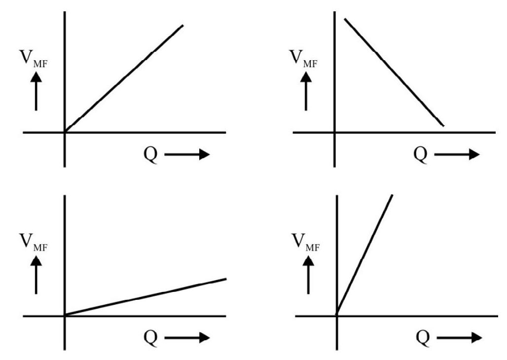
46. A series LCR circuit is connected across a given a.c. source,
(1)
(2)
(3)
(4)
Show Answer
Correct answer: (1)
Solution:
The Q-factor, for a series LCR circuit, equals
The voltage magnification factor, is,
Hence
The graph, between the two, is, therefore, a straight line of slope
Average
Q-factor and Resonant Frequency
47. A sinusoidal A.C. voltage source, of adjustable frequency, is connected across a series ‘LCR’ combination. The inductance
(1)
(2)
(3)
(4)
Show Answer
Correct answer: (2)
Solution:
The resonant frequency,
These give
Average
Phase Angle and Quality Factor in a Series LCR Circuit
48. A voltage source,
(1)
(2)
(3)
(4)
Show Answer
Correct answer: (3)
Solution:
The phase angle,
The quality factor,
Hence, for the given case,
Average
Quality Factor Series LCR Circuits
49. The following table gives the value of
| Circuits No. | Value | |||
|---|---|---|---|---|
| C | ||||
| 1. | ||||
| 2. | ||||
| 3. |
The quality factors,
(1)
(2)
(3)
(4)
Show Answer
Correct answer: (3)
Solution:
We know that
Easy
Quality Factor and Resonant Frequency
50. The inductance, capacitance and resistance in a given series LCR circuit, have values of (n) henry,
(1)
(2)
(3)
(4)
Show Answer
Correct answer: (2)
Solution:
The quality factor,
Also the resonant frequency,
[Note: We can check the consistency of these results by noting that
Easy
Sharpness of Resonance of a Series LCR Circuit
51. It is required to improve the sharpness of resonance of a series LCR circuit by a factor of 4. This requirement can be met by
(1) increasing the resistance to 4 times its present value; leaving
(2) increasing the inductance to eight times to present value; decreasing the capacitance by a factor of 2; and leaving
(3) increasing the inductance by a factor of 4 , leaving
(4) decreasing the capacitance by a factor or 4; leaving
Show Answer
Correct answer: (2)
Solution:
The sharpness of resonance, of a series LCR circuit, improves by a factor of 4 when its quality factor goes up by a factor of 4 . Now
It is easy to see that it is only the changes, suggested in option (2), that increase the value of the Q-factor by a factor of 4 .
Hence we can improve the sharpness of resonance by a factor of (4) by following the changes suggested in option(2).
[Note: The sharpness of resonance improves by a factor of 4 when for the same value of the resonant frequency, the band width,
Average
LCR Circuit
52. A series LC circuit is connected across an a.c. voltage source :
(1)
(2)
(3)
(4)
Show Answer
Correct answer: (2)
Solution:
Since
Easy
Behaviour of
53. A student writes the following statements about the ‘inductors’ and the ‘capacitors’.
(a) An inductor behaves almost like an ‘open’ for very low frequency a.c. sources as well as d.c. sources.
(b) A capacitor behaves like an ‘open’ for very low frequency a.c. sources as well as d.c. sources.
(c) For very high frequency a.c. sources, a capacitor behaves as an ‘open’ while an inductor behaves like a ‘short’.
(d) For very law frequency a.c. sources (as well as d.c. sources), an inductor behaves like an ‘open’ while a capacitor behaves like a short.
(1) a
(2) b
(3) c
(4) d
Show Answer
Correct answer: (2)
Solution:
An ‘open’ implies an (almost) infinite impedance while a ‘short’ implies an impedance tending to zero. Now
(i) Impedance of inductor
(ii) Impedance of capacitor
Hence a capacitor behaves in a way opposite to the behaviour of an inductor.
Hence statement (B) is the only ’logically valid’ statement, out of the four given statement.
Average
LC Circuits
54. A circuit is made up of an (almost) pure inductor and an (almost) pure capacitor, connected together. The circuit (i) has a resonance frequency
(1)
(2)
(3)
(4)
Show Answer
Correct answer: (2)
Solution:
Let
In the presence of the gas, of dielectric constant, say, K, the capacitance changes to KC. Hence
Average
Series LCR Circuit
55. When a given (fixed frequency, fixed voltage) a.c. source is connected across a series LCR circuit, the current in the circuit has its maximum value when
(1)
(2)
(3)
(4)
Show Answer
Correct answer: (1)
Solution:
The impedance of a series
Because of the presence of the squared term
Average
LCR Circuit
56. For the LCR series circuit shown here, the peak value of the voltage of the source, the phase difference between the applied voltage and the current flowing, and the power factor of the circuit, equal, respectively.
(1)
(2)
(3) 10 volt;
(4)
Show Answer
Correct answer: (3)
Solution:
The impedance,
Here
and
Phase difference between current and voltage
Difficult
Adjusting the Value of C in a given LCR Circuit
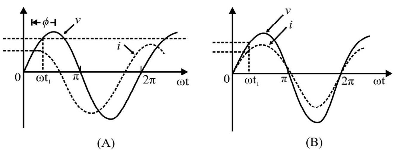
57. The graph drawn here, shows, simultaneously the variation of the (alternating) voltage (applied) and the current (flowing) for a given series LCR circuit.
Without making any other change, the power factor of this circuit, can be made unity if another capacitor,
(1)
(2)
(3)
(4)
Show Answer
Correct answer: (2)
Solution:
The given graph shows the current lagging in phase with respect to the (applied) voltage. The power factor of the circuit becomes unity if the circuit is in its resonance state. This requires the capacitor to have a value, C’, such that
We need to increase the capacitative impedance to make it equal to
This gives
Difficult
Adjusting the Value of L in a given LCR Circuit
58. A given
The current, flowing in this circuit, has to be made to have its maximum value
(1)
(2)
(3)
(4)
Show Answer
Correct answer: (1)
Solution:
The given graph shows the current leading in phase with respect to the applied voltage. The given condition (current has its maximum value
Since the current is leading in phase, we need to increase, the value of the inductance. We, therefore, need to add another inductor (of value L") in series with the given inductor, such that
Average
Changes in LCR Circuit
59. A series
(1)
(2)
(3)
(4)
Show Answer
Correct answer: (4)
Solution:
The phase angle (correct lagging) between the current flowing, and the voltage applied, in a series LCR circuit is given by
Here
Hence
We can make
The required value of
Average
Sereis LCR Circuits
60. A series LCR circuit is connected across a given a.c. voltage source for which
(1)
(2)
(3)
(4)
Show Answer
Correct answer: (1)
Solution:
For the series LCR circuit, (since
Average
Series LCR Circuit
61. The graphs, (A) and (B), drawn here, show, respectively, the phase relationship between the voltage and current, in a series LCR circuit (connectd to an a.c. source) when
(1) (A)
(2) (A)
(3) (A)
(4) (A) alone is shorted (B)
Show Answer
Correct answer: (4)
Solution:
For a series LCR circuit, the (phase) angle
(i) When
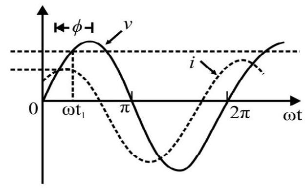
(A)
(ii) When
(B)
[Option (1) and (2) are incorrect becuase when
Average
Resonant Frequency of a Series Combination of Two LCR Circuits
62. The resonance frequency for each of the two individual (LCR) series circuits, [(A) and (B)], shown here, has the same value, say
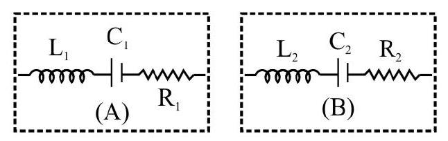
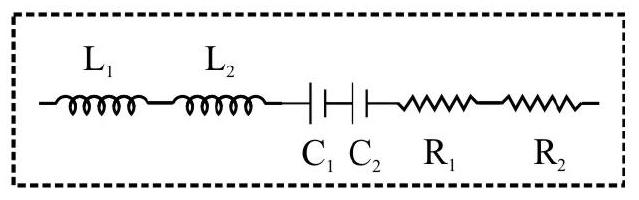
(1)
(2)
(3)
(4)
Show Answer
Correct answer: (1)
Solution:
We are given that
For the ‘combined circuit’, the equivalent inductance (L), and the equivalent capacitance (C), have the values given by
The resonant frequency, say
Now
Average
Phase Angle and Power Factor in a Series LCR Circuit
63. An A.C. voltage source
(1)
(2)
(3)
(4)
Show Answer
Correct answer: (2)
Solution:
The phase angle,
Average
Induced emf
64. A series
(1)
(2)
(3)
(4)
Show Answer
Correct answer: (1)
Solution:
The phase angle (current lagging),
Here
We can make
Average
LCR Circuit
65. A given series LCR circuits is connected across a simusoidal AC voltage source.
The inductance,
(1)
(2)
(3) 0,0 and
(4)
Show Answer
Correct answer: (4)
Solution:
We are given that
Difficult
Adjusting the Value of L in a given LCR Circuit
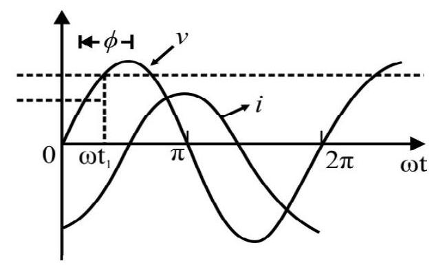
66. A given series LCR circuit has an alternating voltage (
Without making any other change, the value of the (net) inductance, present in the circuit, is to be adjusted such that the voltage of the source, and the voltage drop across the resistor in the circuit, have identical values. For this, we need to put another inductor,
(1)
(2)
(3)
(4)
Show Answer
Correct answer: (3)
Solution:
The voltage of the source, and the voltage drop across the resistor, have identical values only when the circuit is in its resonance state. Hence the net inductance (L’), in the circuit must be such that
Since the current is lagging in phase, the inductance value needs to be decreased. For this, we need to put an inductance
This gives
Difficult
Adjusting the Value of C in a LCR Circuit
67. Graph A, drawn here, shows simulteneously the variation of the (alternating) voltage (applied) and the current (flowing), with time, for a given senses LCR circuit.
Without making any other change in the circuit, the (voltage/current) vs (time) graph, for the circuit, would take the form shown, in graph B, if another capacitor C”, of value
(1)
(2)
(3)
(4)
Show Answer
Correct answer: (1)
Solution:
Graph A shows the current leading in phase w.r.t the voltage. In graph B, the voltage and current are in phase. This means that we need a net value,
Since the current is leading in phase, it can be brought ‘in phase’, by increasing the given value of C. For this, we put a capacitor, C", in parallel with the given capacitance (
Average
LCR Circuits
68. The impedance of a given series LCR circuit, at its resonance (angular) frequency
(1)
(3)
(3)
(4)
Show Answer
Correct answer: (1)
Solution:
The impedance, of a series LCR circuit, at its resonance (angular) frequency
We also have
and
Solving the two equations, we get
and
Difficult
Analysing LCR Circuit
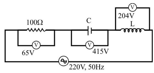
69. An electrical circuit is made up of an inductance (
(1)
(2)
(3)
(4)
Show Answer
Correct answer: (4)
Solution:
Let
Power
Now phase angle,
Here
Also
Also
Hence
Average
Impedance Calculation
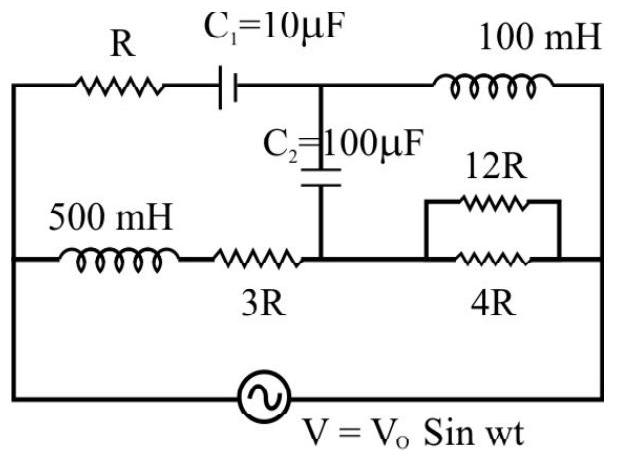
70. The circuit, shown in the figure here, has been connected to an a.c. voltage source
(1)
(2)
(3)
(4)
Show Answer
Correct answer: (1)
Solution:
At very high frequencies, the effective impedance of the capacitor tends to zero while that of the inductor tends to infinity. The branches, containing inductors, are, therefore, (effectively) not parts of the circuit while those conatining the capacitor, are (effectively) like a simple connecting wire. The circuit, therefore, looks effectively like the one shown here.
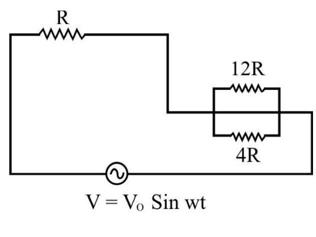
The effective impedance is, therefore,
Average
Induced emf in a Rotating Coil
71. A planar circular coil, of radius
(1) an external torque, of magnitude
(2) an external torque, of magnitude
(3) an external torque, of magnitude
(4) it just needs to be given the necessary ‘spin’ at start, it would then keep on rotating at its initial rate, due to its ‘rotational inertia’.
Show Answer
Correct answer: (2)
Solution:
Let the coil rotate about a diameter, taken as the
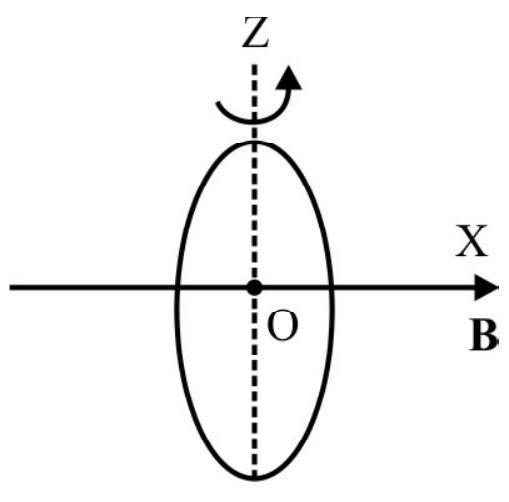
Instantaneous induced current
The magnetic moment, associated with this induced current,
The magnetic field exerts a torque, which has an instantneous value,
The external torque is needed to oppose this torque on the coil due to the induced current. Hence external torque
Average
AC Generator
72. A circular coil, having
The magnitudes of the instantaneous emf, induced in the coil, when its plane
(i) is at right angles to the magnetic meridian.
(ii) makes an angle of
(iii) coincides with the magnetic merician, would equal, respectively.
(1)
(2)
(3)
(4)
Show Answer
Correct answer: (1)
Solution:
When the normal, to the plane of the coil, makes an angle
In the cases (i), (ii), (iii),
Hence the three values of
Average
AC Generator
73. A mini generator has a coil of 1000 turns, each of area
(1) 0 volt, 0 volt, 0 volt, 0 volt
(2) 0 volt, 100 volt, 0 volt, 100 volt
(3) 100 volt, 0 volt, 100 volt, 0 volt
(4) 100 volt, 100 volt, 100 volt, 100 volt
Show Answer
Correct answer: (4)
Solution:
The flux, linked with the coil, at any instant is
Here
The average, of this, over success four quarters of the cycle, are given by
Easy
Transformer
74. A step down transformer (having windings of negligible resistance) is used to step down the mains voltage of
(1)
(2)
(3)
(4)
Show Answer
Correct answer: (3)
Solution:
The secondary, supplying a voltage of
Hence current in the secondary
Efficiency
Power available in the primary circuit
Average
Transformer
75. The diagram, given here, shows a ‘step-up’ that may be used to supply power from a ‘power plant’ to a ’town’ via transmission lines of a total (to and fro) length of
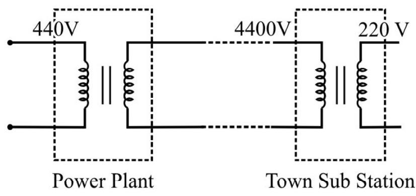
(1)
(2)
(3)
(4)
Show Answer
Correct answer: (4)
Solution:
The power available at the primary coil of the town substation transformer = power requirement of town
Voltage available at its primary
Total resistance of the line
Voltage drop across the line
Average
Transformer
76. A power station, located at a distance of
The power station uses a step-up transformer to boost the voltage to
(1)
(2)
(3)
(4)
Show Answer
Correct answer: (2)
Solution:
The total resistance, of the transmission lines, is
The current in the transmission wires
Average
RMS Value
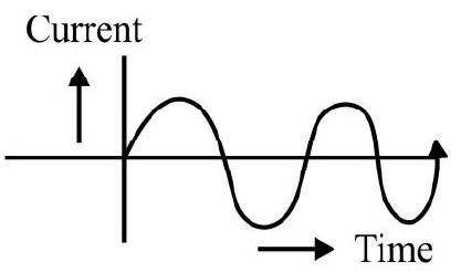
77. The alternating current, in a given set up, varies with time in the manner shown. The rms value of this current, over one cycle, is
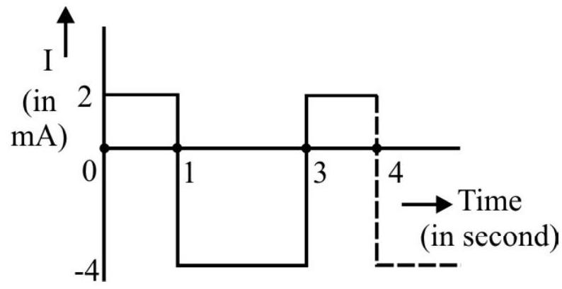
(1)
(2)
(3)
(4)
Show Answer
Correct answer: (2)
Solution:
The rms value, by definition, is obtained by taking the average of the squares of all values (over one complete cycle) and then taking the square root of this average.
For the given case, we have
For
For
For
Difficult
Voltage (in Volt)
78. The rms value, of the saw tooth alternating voltage, shown here, equals (nearly)
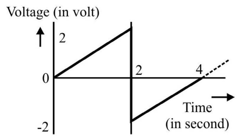
(1) 1.732 Volt
(2) 1.00 Volt
(3) 1.15 Volt
(4) 1.42 Volt
Show Answer
Correct answer: (3)
Solution:
The rms value, by definition, is obtained by taking the average of the squares of all values (over one complete cycle) and then taking the square root of this average.
We see that for the time period of the alternating voltage is
For
For
Average
Induced Current and Resulting Power Loss
79. A circular coil, of radius
(1)
(2)
(3)
(4)
Show Answer
Correct answer: (2)
Solution:
The instantaneous flux, linked with the coil; is
where
Easy
Wattless Curents
80. For a pure inductor, or a pure capacitor, connected to an a.c. voltage source, one can say that the instantnaeous power.
(1) as well as the average, over a cycle, are both zero
(2) may not be zero but the average power, over a cycle, is zero
(3) can zero but the average power, over a cycle, is hot zero
(4) as well as the average power, over a cycle, are both not zero
Show Answer
Correct answer: (2)
Solution:
The current, in a pure inductor, or a pure capacitor, has a phase lag of
This is not zero at all instant. However, its average, over a complete cycle, is zero.


