7.1 INTRODUCTION

We have so far considered direct current (dc) sources and circuits with dc sources. These currents do not change direction with time. But voltages and currents that vary with time are very common. The electric mains supply in our homes and offices is a voltage that varies like a sine function with time. Such a voltage is called alternating voltage (ac voltage) and the current driven by it in a circuit is called the alternating current (ac current)*. Today, most of the electrical devices we use require ac voltage. This is mainly because most of the electrical energy sold by power companies is transmitted and distributed as alternating current. The main reason for preferring use of ac voltage over dc voltage is that ac voltages can be easily and efficiently converted from one voltage to the other by means of transformers. Further, electrical energy can also be transmitted economically over long distances. AC circuits exhibit characteristics which are exploited in many devices of daily use. For example, whenever we tune our radio to a favourite station, we are taking advantage of a special property of ac circuits - one of many that you will study in this chapter.

FIGURE 7.2 In a pure resistor, the voltage and current are in phase. The minima, zero and maxima occur at the same respective times.

7.2 AC Voltage Applied to a Resistor

Figure 7.1 shows a resistor connected to a source $\varepsilon$ of ac voltage. The symbol for an ac source in a circuit diagram is $\Theta$. We consider a source which produces sinusoidally varying potential difference across its terminals. Let this potential difference, also called ac voltage, be given by

$$ \begin{equation*} v=v_{m} \sin \omega t \tag{7.1} \end{equation*} $$

FIGURE 7.1 AC voltage applied to a resistor.

where $v_{m}$ is the amplitude of the oscillating potential difference and $\omega$ is its angular frequency.

To find the value of current through the resistor, we apply Kirchhoffs loop rule $\sum \varepsilon(t)=0$ (refer to Section 3.13), to the circuit shown in Fig. 7.1 to get

$$ v_{m} \sin \omega t=i R $$

or $i=\frac{v_{m}}{R} \sin \omega t$

Since $R$ is a constant, we can write this equation as

$$ \begin{equation*} i=i_{m} \sin \omega t \tag{7.2} \end{equation*} $$

where the current amplitude $i_{m}$ is given by

$$ \begin{equation*} i_{m}=\frac{v_{m}}{R} \tag{7.3} \end{equation*} $$

FIGURE 7.2 In a pure resistor, the voltage and current are in phase. The minima, zero and maxima occur at the same respective times.

Equation (7.3) is Ohm’s law, which for resistors, works equally well for both ac and dc voltages. The voltage across a pure resistor and the current through it, given by Eqs. (7.1) and (7.2) are plotted as a function of time in Fig. 7.2. Note, in particular that both $v$ and $i$ reach zero, minimum and maximum values at the same time. Clearly, the voltage and current are in phase with each other.

We see that, like the applied voltage, the current varies sinusoidally and has corresponding positive and negative values during each cycle. Thus, the sum of the instantaneous current values over one complete cycle is zero, and the average current is zero. The fact that the average current is zero, however, does not mean that the average power consumed is zero and that there is no dissipation of electrical energy. As you know, Joule heating is given by $i^{2} R$ and depends on $i^{2}$ (which is always positive whether $i$ is positive or negative) and not on $i$. Thus, there is Joule heating and dissipation of electrical energy when an ac current passes through a resistor.

The instantaneous power dissipated in the resistor is

$$ \begin{equation*} p=i^{2} R=i_{m}^{2} R \sin ^{2} \omega t \tag{7.4} \end{equation*} $$

The average value of $p$ over a cycle is*

$$ \begin{equation*} \bar{p}=<i^{2} R>=<i_{m}^{2} R \sin ^{2} \omega t> \tag{a} \end{equation*} $$

where the bar over a letter (here, $p$ ) denotes its average value and $<\ldots . .>$ denotes taking average of the quantity inside the bracket. Since, $i_{m}^{2}$ and $R$ are constants,

$$ \begin{equation*} \bar{p}=i_{m}^{2} R<\sin ^{2} \omega t> \tag{b} \end{equation*} $$

Using the trigonometric identity, $\sin ^{2} \omega t=$ $1 / 2(1-\cos 2 \omega t)$, we have $\left.<\sin ^{2} \omega t>=(1 / 2)(1-<\cos 2 \omega t \right)$ and since $<\cos 2 \omega t>=0^{*}$, we have,

$$ <\sin ^{2} \omega t>=\frac{1}{2} $$

Thus,

$$ \begin{equation*} \bar{p}=\frac{1}{2} i_{m}^{2} R \tag{c} \end{equation*} $$

To express ac power in the same form as dc power $\left(P=I^{2} R\right)$, a special value of current is defined and used. It is called, root mean square (rms) or effective current (Fig. 7.3) and is denoted by $I_{r m s}$ or $I$.

FIGURE 7.3 The rms current $I$ is related to the peak current $i_{m}$ by $I=i_{m} / \sqrt{2}=0.707 i_{m}$.

• The average value of a function $F(t)$ over a period $T$ is given by $\langle F(t)\rangle=\frac{1}{T} \int_{0}^{T} F(t) \mathrm{d} t$

$<\cos 2 \omega t> \text{=} \frac{1}{T} \int_{0}^{T}\cos 2 \omega tdt \text{=} \frac{1}{T}[\large\frac{\sin 2 \omega t}{2 \omega}]_{0}^{T} \text{=}\frac{1}{2 \omega T}[\sin 2 \omega \text{-}0]=0$

It is defined by

$$ \begin{align*} I=\sqrt{\overline{i^{2}}} & =\sqrt{\frac{1}{2} i_{m}^{2}}=\frac{i_{m}}{\sqrt{2}} \\ & =0.707 i_{m} \tag{7.6} \end{align*} $$

In terms of $I$, the average power, denoted by $P$ is

$$ \begin{equation*} P=\bar{p}=\frac{1}{2} i_{m}^{2} R=I^{2} R \tag{7.7} \end{equation*} $$

Similarly, we define the rms voltage or effective voltage by

$$ \begin{equation*} V=\frac{v_{m}}{\sqrt{2}}=0.707 v_{m} \tag{7.8} \end{equation*} $$

From Eq. (7.3), we have

$$ v_{m}=i_{m} R $$

or, $\frac{v_{m}}{\sqrt{2}}=\frac{i_{m}}{\sqrt{2}} R$

or, $V=I R$

Equation (7.9) gives the relation between ac current and ac voltage and is similar to that in the dc case. This shows the advantage of introducing the concept of rms values. In terms of rms values, the equation for power [Eq. (7.7)] and relation between current and voltage in ac circuits are essentially the same as those for the dc case.

It is customary to measure and specify rms values for ac quantities. For example, the household line voltage of $220 \mathrm{~V}$ is an $\mathrm{rms}$ value with a peak voltage of

$$ v_{m}=\sqrt{2} \quad V=(1.414)(220 \mathrm{~V})=311 \mathrm{~V} $$

In fact, the $I$ or rms current is the equivalent dc current that would produce the same average power loss as the alternating current. Equation (7.7) can also be written as

$$ P=V^{2} / R=I V \quad(\text { since } V=I R) $$

7.3 Representation of AC Current and Voltage by Rotating Vectors - Phasors

In the previous section, we learnt that the current through a resistor is in phase with the ac voltage. But this is not so in the case of an inductor, a capacitor or a combination of these circuit elements. In order to show phase relationship between voltage and current in an ac circuit, we use the notion of phasors. The analysis of an ac circuit is facilitated by the use of a phasor diagram. A phasor* is a vector which rotates about the origin with angular speed $\omega$, as shown in Fig. 7.4. The vertical components of phasors $\mathbf{V}$ and $\mathbf{I}$ represent the sinusoidally varying quantities $v$ and $i$. The magnitudes of phasors $\mathbf{V}$ and $\mathbf{I}$ represent the amplitudes or the peak values $v_{m}$ and $i_{m}$ of these oscillating quantities. Figure 7.4(a) shows the voltage and current phasors and their relationship at time $t_{1}$ for the case of an ac source

FIGURE 7.4 (a) A phasor diagram for the circuit in Fig 7.1. (b) Graph of $v$ and $i$ versus $\omega t$.

connected to a resistor i.e., corresponding to the circuit shown in Fig. 7.1. The projection of voltage and current phasors on vertical axis, i.e., $v_{m} \sin \omega t$ and $i_{m} \sin \omega t$, respectively represent the value of voltage and current at that instant. As they rotate with frequency $\omega$, curves in Fig. 7.4(b) are generated.

From Fig. 7.4(a) we see that phasors $\mathbf{V}$ and $\mathbf{I}$ for the case of a resistor are in the same direction. This is so for all times. This means that the phase angle between the voltage and the current is zero.

7.4 AC Voltage Applied to an Inductor

Figure 7.5 shows an ac source connected to an inductor. Usually, inductors have appreciable resistance in their windings, but we shall assume that this inductor has negligible resistance. Thus, the circuit is a purely inductive ac circuit. Let the voltage across the source be $v=v_{m} \sin \omega t$. Using the Kirchhoff’s loop rule, $\sum \varepsilon(t)=0$, and since there is no resistor in the circuit,

$$ \begin{equation*} v-L \frac{\mathrm{d} i}{\mathrm{~d} t}=0 \tag{7.10} \end{equation*} $$

where the second term is the self-induced Faraday emf in the inductor; and $L$ is the self-inductance of

FIGURE 7.5 An ac source connected to an inductor.[^1]the inductor. The negative sign follows from Lenz’s law (Chapter 6). Combining Eqs. (7.1) and (7.10), we have

$$ \begin{equation*} \frac{\mathrm{d} i}{\mathrm{~d} t}=\frac{v}{L}=\frac{v_{m}}{L} \sin \omega t \tag{7.11} \end{equation*} $$

Equation (7.11) implies that the equation for $i(t)$, the current as a function of time, must be such that its slope $\mathrm{d} i / \mathrm{d} t$ is a sinusoidally varying quantity, with the same phase as the source voltage and an amplitude given by $v_{m} / L$. To obtain the current, we integrate $\mathrm{d} i / \mathrm{d} t$ with respect to time:

$$ \int \frac{\mathrm{d} i}{\mathrm{~d} t} \mathrm{~d} t=\frac{v_{m}}{L} \int \sin (\omega t) \mathrm{d} t $$

and get,

$$ i=-\frac{v_{m}}{\omega L} \cos (\omega t)+\text { constant } $$

The integration constant has the dimension of current and is timeindependent. Since the source has an emf which oscillates symmetrically about zero, the current it sustains also oscillates symmetrically about zero, so that no constant or time-independent component of the current exists. Therefore, the integration constant is zero.

Using

$$ -\cos (\omega t)=\sin \omega t-\frac{\pi}{2} \text {, we have } $$

$$ \begin{equation*} i=i_{m} \sin \omega t-\frac{\pi}{2} \tag{7.12} \end{equation*} $$

where $i_{m}=\frac{v_{m}}{\omega L}$ is the amplitude of the current. The quantity $\omega L$ is analogous to the resistance and is called inductive reactance, denoted by $X_{L}$ :

$$ \begin{equation*} X_{L}=\omega L \tag{7.13} \end{equation*} $$

The amplitude of the current is, then

$$ \begin{equation*} i_{m}=\frac{v_{m}}{X_{L}} \tag{7.14} \end{equation*} $$

The dimension of inductive reactance is the same as that of resistance and its SI unit is ohm $(\Omega)$. The inductive reactance limits the current in a purely inductive circuit in the same way as the resistance limits the current in a purely resistive circuit. The inductive reactance is directly proportional to the inductance and to the frequency of the current.

A comparison of Eqs. (7.1) and (7.12) for the source voltage and the current in an inductor shows that the current lags the voltage by $\pi / 2$ or one-quarter (1/4) cycle. Figure 7.6 (a) shows the voltage and the current phasors in the present case at instant $t_{1}$. The current phasor $\mathbf{I}$ is $\pi / 2$ behind the voltage phasor $\mathbf{V}$. When rotated with frequency $\omega$ counterclockwise, they generate the voltage and current given by Eqs. (7.1) and (7.12), respectively and as shown in Fig. 7.6(b).

FIGURE 7.6 (a) A Phasor diagram for the circuit in Fig. 7.5.

(b) Graph of $v$ and $i$ versus $\omega t$.

We see that the current reaches its maximum value later than the voltage by one-fourth of a period $\frac{T}{4}=\frac{\pi / 2}{\omega}$. You have seen that an inductor has reactance that limits current similar to resistance in a dc circuit. Does it also consume power like a resistance? Let us try to find out.

The instantaneous power supplied to the inductor is

$$ \begin{aligned} p_{L}=i v & =i_{m} \sin \omega t-\frac{\pi}{2} \times v_{m} \sin (\omega t) \\ & =-i_{m} v_{m} \cos (\omega t) \sin (\omega t) \\ & =-\frac{i_{m} v_{m}}{2} \sin (2 \omega t) \end{aligned} $$

So, the average power over a complete cycle is

$$ \begin{aligned} P_{\mathrm{L}} & =\left\langle-\frac{i_{m} v_{m}}{2} \sin (2 \omega t)\right\rangle \\ & =-\frac{i_{m} v_{m}}{2}\langle\sin (2 \omega t)\rangle=0 \end{aligned} $$

since the average of $\sin (2 \omega t)$ over a complete cycle is zero.

Thus, the average power supplied to an inductor over one complete cycle is zero.

7.5 AC Voltage Applied to a Capacitor

Figure 7.7 shows an ac source $\varepsilon$ generating ac voltage $v=v_{m}$ sin $\omega \mathrm{t}$ connected to a capacitor only, a purely capacitive ac circuit.

When a capacitor is connected to a voltage source

FIGURE 7.7 An ac source connected to a capacitor. in a dc circuit, current will flow for the short time required to charge the capacitor. As charge accumulates on the capacitor plates, the voltage across them increases, opposing the current. That is, a capacitor in a dc circuit will limit or oppose the current as it charges. When the capacitor is fully charged, the current in the circuit falls to zero.

When the capacitor is connected to an ac source, as in Fig. 7.7, it limits or regulates the current, but does not completely prevent the flow of charge. The capacitor is alternately charged and discharged as the current reverses each half cycle. Let $q$ be the charge on the capacitor at any time $t$. The instantaneous voltage $v$ across the capacitor is

$$ \begin{equation*} v=\frac{q}{C} \tag{7.15} \end{equation*} $$

From the Kirchhoff’s loop rule, the voltage across the source and the capacitor are equal,

$$ v_{m} \sin \omega t=\frac{q}{C} $$

To find the current, we use the relation $i=\frac{\mathrm{d} q}{\mathrm{~d} t}$

$$ i=\frac{\mathrm{d}}{\mathrm{d} t}\left(v_{m} C \sin \omega t\right)=\omega C v_{m} \cos (\omega t) $$

Using the relation, $\cos (\omega t)=\sin \omega t+\frac{\pi}{2}$, we have

$$ \begin{equation*} i=i_{m} \sin \omega t+\frac{\pi}{2} \tag{7.16} \end{equation*} $$

where the amplitude of the oscillating current is $i_{m}=\omega C v_{m}$. We can rewrite it as

$$ i_{m}=\frac{v_{m}}{(1 / \omega C)} $$

Comparing it to $i_{m}=v_{m} / R$ for a purely resistive circuit, we find that $(1 / \omega C)$ plays the role of resistance. It is called capacitive reactance and is denoted by $X_{c}$,

$$ \begin{equation*} X_{c}=1 / \omega C \tag{7.17} \end{equation*} $$

so that the amplitude of the current is

$$ \begin{equation*} i_{m}=\frac{v_{m}}{X_{C}} \tag{7.18} \end{equation*} $$

The dimension of capacitive reactance is the same as that of resistance and its SI unit is ohm $(\Omega)$. The capacitive reactance limits the amplitude of the current in a purely capacitive circuit in the same way as the resistance limits the current in a purely resistive circuit. But it is inversely proportional to the frequency and the capacitance.

A comparison of Eq. (7.16) with the equation of source voltage, Eq. (7.1) shows that the current is $\pi / 2$ ahead of voltage.

Figure 7.8(a) shows the phasor diagram at an instant $t_{1}$. Here the current phasor $\mathbf{I}$ is $\pi / 2$ ahead of the voltage phasor $\mathbf{V}$ as they rotate counterclockwise. Figure 7.8(b) shows the variation of voltage and current with time. We see that the current reaches its maximum value earlier than the voltage by one-fourth of a period.

The instantaneous power supplied to the capacitor is

$$ \begin{align*} p_{c} & =i v=i_{m} \cos (\omega t) v_{m} \sin (\omega t) \\ & =i_{m} v_{m} \cos (\omega t) \sin (\omega t) \\ & =\frac{i_{m} v_{m}}{2} \sin (2 \omega t) \tag{7.19} \end{align*} $$

So, as in the case of an inductor, the average power

$$ P_{C}=\left\langle\frac{i_{m} v_{m}}{2} \sin (2 \omega t)\right\rangle=\frac{i_{m} v_{m}}{2}\langle\sin (2 \omega t)\rangle=0 $$

since $<\sin (2 \omega t)>=0$ over a complete cycle.

Thus, we see that in the case of an inductor, the current lags the voltage by $\pi / 2$ and in the case of a capacitor, the current leads the voltage by $\pi / 2$.

7.6 AC Voltage Applied to a Series LCR Circuit

Figure 7.10 shows a series LCR circuit connected to an ac source $\varepsilon$. As

usual, we take the voltage of the source to be $v=v_{m} \sin \omega t$.

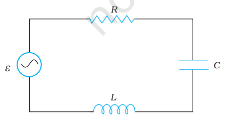
FIGURE 7.10 A series LCR circuit connected to an ac source.

If $q$ is the charge on the capacitor and $i$ the current, at time $t$, we have, from Kirchhoff’s loop rule:

$$ \begin{equation*} L \frac{\mathrm{d} i}{\mathrm{~d} t}+i R+\frac{q}{C}=v \tag{7.20} \end{equation*} $$

We want to determine the instantaneous current $i$ and its phase relationship to the applied alternating voltage $v$. We shall solve this problem by two methods. First, we use the technique of phasors and in the second method, we solve Eq. (7.20) analytically to obtain the timedependence of $i$.

7.6.1 Phasor-diagram solution

From the circuit shown in Fig. 7.10, we see that the resistor, inductor and capacitor are in series. Therefore, the ac current in each element is the same at any time, having the same amplitude and phase. Let it be

$$ \begin{equation*} i=i_{m} \sin (\omega t+\phi) \tag{7.21} \end{equation*} $$

where $\phi$ is the phase difference between the voltage across the source and the current in the circuit. On the basis of what we have learnt in the previous sections, we shall construct a phasor diagram for the present case.

Let $\mathbf{I}$ be the phasor representing the current in the circuit as given by Eq. (7.21). Further, let $\mathbf{V_\mathbf{L}}, \mathbf{V_\mathbf{R}}, \mathbf{V_\mathbf{C}}$, and $\mathbf{V}$ represent the voltage across the inductor, resistor, capacitor and the source, respectively. From previous section, we know that $\mathbf{V_\mathbf{R}}$ is parallel to $\mathbf{I}, \mathbf{V_\mathbf{C}}$ is $\pi / 2$ behind $\mathbf{I}$ and $\mathbf{V_\mathbf{L}}$ is $\pi / 2$ ahead of $\mathbf{I}$. $\mathbf{V_\mathbf{L}}, \mathbf{V_\mathbf{R}}, \mathbf{V_\mathbf{C}}$ and $\mathbf{I}$ are shown in Fig. 7.11(a) with apppropriate phaserelations.

The length of these phasors or the amplitude of $\mathbf{v_\mathbf{R}}, \mathbf{v_\mathbf{C}}$ and $\mathbf{v_\mathbf{L}}$ are:

$$ \begin{equation*} v_{R m}=i_{m} R, v_{C m}=i_{m} X_{C}, v_{L m}=i_{m} X_{L} \tag{7.22} \end{equation*} $$

The voltage Equation (7.20) for the circuit can be written as

$$ \begin{equation*} v_{\mathrm{L}}+v_{\mathrm{R}}+v_{\mathrm{C}}=v \tag{7.23} \end{equation*} $$

The phasor relation whose vertical component gives the above equation is

$$ \begin{equation*} \mathbf{v_\mathrm{L}}+\mathbf{v_\mathrm{R}}+\mathbf{v_\mathrm{C}}=\mathbf{V} \tag{7.24} \end{equation*} $$

This relation is represented in Fig. 7.11(b). Since

FIGURE 7.11 (a) Relation between the phasors $\mathbf{V_\mathrm{L}}, \mathbf{v_\mathrm{R}}, \mathbf{v_\mathrm{C}}$, and $I$, (b) Relation between the phasors $\mathbf{V_\mathrm{L}}, \mathbf{V_\mathrm{R}}$, and $\left(\mathbf{V_\mathrm{L}}+\mathbf{V_\mathrm{C}}\right)$ for the circuit in Fig. 7.10. $\mathbf{V_\mathbf{C}}$ and $\mathbf{V_\mathbf{L}}$ are always along the same line and in opposite directions, they can be combined into a single phasor $\left(\mathbf{V_\mathbf{C}}+\mathbf{V_\mathbf{L}}\right)$ which has a magnitude $\left|v_{C m}-v_{L m}\right|$. Since $\mathbf{V}$ is represented as the hypotenuse of a right-triangle whose sides are $\mathbf{V_\mathbf{R}}$ and $\left(\mathbf{V_\mathbf{C}}+\mathbf{V_\mathbf{L}}\right)$, the pythagorean theorem gives:

$$ v_{m}^{2}=v_{R m}^{2}+\left(v_{C m}-v_{L m}\right)^{2} $$

Substituting the values of $v_{R m}, v_{C m}$, and $v_{L m}$ from Eq. (7.22) into the above equation, we have

$$ \begin{aligned} v_{m}^{2} & =\left(i_{m} R\right)^{2}+\left(i_{m} X_{C}-i_{m} X_{L}\right)^{2} \\ & =i_{m}^{2} \quad R^{2}+\left(X_{C}-X_{L}\right)^{2} \end{aligned} $$

or, $i_{m}=\frac{v_{m}}{\sqrt{R^{2}+\left(X_{C}-X_{L}\right)^{2}}}$

By analogy to the resistance in a circuit, we introduce the impedance $Z$ in an ac circuit:

$$ \begin{equation*} i_{m}=\frac{v_{m}}{Z} \tag{b} \end{equation*} $$

where $Z=\sqrt{R^{2}+\left(X_{C}-X_{L}\right)^{2}}$

FIGURE 7.12 Impedance diagram.

Since phasor $\mathbf{I}$ is always parallel to phasor $\mathbf{V_\mathbf{R}}$, the phase angle $\phi$ is the angle between $\mathbf{V_\mathbf{R}}$ and $\mathbf{V}$ and can be determined from Fig. 7.12:

$\tan \varphi=\frac{v_{C m}-v_{L m}}{v_{R m}}$

Using Eq. (7.22), we have

$\tan \varphi=\frac{X_{C}-X_{L}}{R}$

Equations (7.26) and (7.27) are graphically shown in Fig. (7.12). This is called Impedance diagram which is a right-triangle with $Z$ as its hypotenuse.

Equation 7.25(a) gives the amplitude of the current and Eq. (7.27) gives the phase angle. With these, Eq. (7.21) is completely specified.

If $X_{C}>X_{L}, \phi$ is positive and the circuit is predominantly capacitive. Consequently, the current in the circuit leads the source voltage. If $X_{C}<X_{L}, \phi$ is negative and the circuit is predominantly inductive. Consequently, the current in the circuit lags the source voltage.

Figure 7.13 shows the phasor diagram and variation of $v$ and $i$ with $\omega t$ for the case $X_{C}>X_{L}$.

(a) (b) FIGURE 7.13 (a) Phasor diagram of $\mathbf{V}$ and $\mathbf{I}$.

(b) Graphs of $v$ and $i$ versus $\omega t$ for a series LCR circuit where $X_{C}>X_{L}$. Thus, we have obtained the amplitude and phase of current for an $L C R$ series circuit using the technique of phasors. But this method of analysing ac circuits suffers from certain disadvantages. First, the phasor diagram say nothing about the initial condition. One can take any arbitrary value of $t$ (say, $t_{1}$, as done throughout this chapter) and draw different phasors which show the relative angle between different phasors. The solution so obtained is called the steady-state solution. This is not a general solution. Additionally, we do have a transient solution which exists even for $v=0$. The general solution is the sum of the transient solution and the steady-state solution. After a sufficiently long time, the effects of the transient solution die out and the behaviour of the circuit is described by the steady-state solution.

7.6.2 Resonance

An interesting characteristic of the series RLC circuit is the phenomenon of resonance. The phenomenon of resonance is common among systems that have a tendency to oscillate at a particular frequency. This frequency is called the system’s natural frequency. If such a system is driven by an energy source at a frequency that is near the natural frequency, the amplitude of oscillation is found to be large. A familiar example of this for swinging back and forth like a pendulum. If the child pulls on the rope at regular intervals and the frequency of the pulls is almost the same as the frequency of swinging, the amplitude of the swinging will be large (Chapter 13, Class XI).

For an $R L C$ circuit driven with voltage of amplitude $v_{m}$ and frequency $\omega$, we found that the current amplitude is given by

$$ i_{m}=\frac{v_{m}}{Z}=\frac{v_{m}}{\sqrt{R^{2}+\left(X_{C}-X_{L}\right)^{2}}} $$

with $X_{c}=1 / \omega C$ and $X_{L}=\omega L$. So if $\omega$ is varied, then at a particular frequency $\omega_{0}, X_{c}=X_{L}$, and the impedance is minimum $\left(Z=\sqrt{R^{2}+0^{2}}=R\right)$. This frequency is called the resonant frequency:

$$ X_{c}=X_{L} \text { or } \frac{1}{\omega_{0} C}=\omega_{0} L $$

or $\omega_{0}=\frac{1}{\sqrt{L C}}$

At resonant frequency, the current amplitude is maximum; $i_{m}=v_{m} / R$.

Figure 7.16 shows the variation of $i_{m}$ with $\omega$ in a $R L C$ series circuit with $L=1.00 \mathrm{mH}, C=$ $1.00 \mathrm{nF}$ for two values of $R$ : (i) $R=100 \Omega$ and (ii) $R=200 \Omega$. For the source applied $v_{m}=$

100 V. $\omega_{0}$ for this case is $\frac{1}{\sqrt{L C}}=1.00 \times 10^{6}$ $\mathrm{rad} / \mathrm{s}$.

We see that the current amplitude is maximum at the resonant frequency. Since $i_{m}=$

FIGURE 7.14 Variation of $i_{m}$ with $\omega$ for two cases: (i) $R=100 \Omega$, (ii) $R=200 \Omega$, $L=1.00 \mathrm{mH}$. $v_{m} / R$ at resonance, the current amplitude for case (i) is twice to that for case (ii).

Resonant circuits have a variety of applications, for example, in the tuning mechanism of a radio or a TV set. The antenna of a radio accepts signals from many broadcasting stations. The signals picked up in the antenna acts as a source in the tuning circuit of the radio, so the circuit can be driven at many frequencies. But to hear one particular radio station, we tune the radio. In tuning, we vary the capacitance of a capacitor in the tuning circuit such that the resonant frequency of the circuit becomes nearly equal to the frequency of the radio signal received. When this happens, the amplitude of the current with the frequency of the signal of the particular radio station in the circuit is maximum.

It is important to note that resonance phenomenon is exhibited by a circuit only if both $L$ and $C$ are present in the circuit. Only then do the voltages across $L$ and $C$ cancel each other (both being out of phase) and the current amplitude is $v_{m} / R$, the total source voltage appearing across $R$. This means that we cannot have resonance in a RL or $R C$ circuit.

7.7 Power in AC Circuit: The Power Factor

We have seen that a voltage $v=v_{m} \sin \omega t$ applied to a series $R L C$ circuit drives a current in the circuit given by $i=i_{m} \sin (\omega t+\phi)$ where

$$ i_{m}=\frac{v_{m}}{Z} \text { and } \phi=\tan ^{-1} \frac{X_{C}-X_{L}}{R} $$

Therefore, the instantaneous power $p$ supplied by the source is

$$ \begin{align*} & p=v i=\left(v_{m} \sin \omega t\right) \times\left[i_{m} \sin (\omega t+\varphi)\right] \\ & =\frac{v_{m} i_{m}}{2}[\cos \varphi-\cos (2 \omega t+\varphi)] \tag{7.29} \end{align*} $$

The average power over a cycle is given by the average of the two terms in R.H.S. of Eq. (7.37). It is only the second term which is time-dependent. Its average is zero (the positive half of the cosine cancels the negative half). Therefore,

$$ \begin{align*} & P=\frac{v_{m} i_{m}}{2} \cos \varphi=\frac{v_{m}}{\sqrt{2}} \frac{i_{m}}{\sqrt{2}} \cos \varphi \\ & =V I \cos \varphi \tag{a} \end{align*} $$

This can also be written as,

$$ \begin{equation*} P=I^{2} Z \cos \varphi \tag{b} \end{equation*} $$

So, the average power dissipated depends not only on the voltage and current but also on the cosine of the phase angle $\phi$ between them. The quantity $\cos \phi$ is called the power factor. Let us discuss the following cases:

Case (i) Resistive circuit: If the circuit contains only pure $R$, it is called resistive. In that case $\phi=0, \cos \phi=1$. There is maximum power dissipation.

Case (ii) Purely inductive or capacitive circuit: If the circuit contains only an inductor or capacitor, we know that the phase difference between voltage and current is $\pi / 2$. Therefore, $\cos \phi=0$, and no power is dissipated even though a current is flowing in the circuit. This current is sometimes referred to as wattless current.

Case (iii) $L C R$ series circuit: In an LCR series circuit, power dissipated is given by Eq. (7.30) where $\phi=\tan ^{-1}\left(X_{c}-X_{L}\right) / R$. So, $\phi$ may be non-zero in a $R L$ or $R C$ or $R C L$ circuit. Even in such cases, power is dissipated only in the resistor.

Case (iv) Power dissipated at resonance in LCR circuit: At resonance $X_{c}-X_{L}=0$, and $\phi=0$. Therefore, $\cos \phi=1$ and $P=I^{2} Z=I^{2} R$. That is, maximum power is dissipated in a circuit (through $R$ ) at resonance.

7.8 TRANSFORMERS

For many purposes, it is necessary to change (or transform) an alternating voltage from one to another of greater or smaller value. This is done with a device called transformer using the principle of mutual induction.

A transformer consists of two sets of coils, insulated from each other. They are wound on a soft-iron core, either one on top of the other as in Fig. 7.16(a) or on separate limbs of the core as in Fig. 7.16(b). One of the coils called the primary coil has $N_{p}$ turns. The other coil is called the secondary coil; it has $N_{s}$ turns. Often the primary coil is the input coil and the secondary coil is the output coil of the transformer.

FIGURE 7.16 Two arrangements for winding of primary and secondary coil in a transformer: (a) two coils on top of each other, (b) two coils on separate limbs of the core.

When an alternating voltage is applied to the primary, the resulting current produces an alternating magnetic flux which links the secondary and induces an emf in it. The value of this emf depends on the number of turns in the secondary. We consider an ideal transformer in which the primary has negligible resistance and all the flux in the core links both primary and secondary windings. Let $\phi$ be the flux in each turn in the core at time $t$ due to current in the primary when a voltage $v_{p}$ is applied to it.

Then the induced emf or voltage $\varepsilon_{s}$, in the secondary with $N_{s}$ turns is

$$ \begin{equation*} \varepsilon_{\mathrm{s}}=-N_{\mathrm{s}} \frac{\mathrm{d} \varphi}{\mathrm{d} t} \tag{7.31} \end{equation*} $$

The alternating flux $\phi$ also induces an emf, called back emf in the primary. This is

$$ \begin{equation*} \varepsilon_{p}=-N_{p} \frac{\mathrm{d} \varphi}{\mathrm{d} t} \tag{7.32} \end{equation*} $$

But $\varepsilon_{p}=v_{p}$. If this were not so, the primary current would be infinite since the primary has zero resistance (as assumed). If the secondary is an open circuit or the current taken from it is small, then to a good approximation

$$ \varepsilon_{s}=v_{s} $$

where $v_{s}$ is the voltage across the secondary. Therefore, Eqs. (7.31) and (7.32) can be written as

$$ \begin{align*} & v_{s}=-N_{s} \frac{d \varphi}{d t} \tag{a}\\ & v_{p}=-N_{p} \frac{d \varphi}{d t} \tag{a} \end{align*} $$

From Eqs. [7.31 (a)] and [7.32 (a)], we have

$$ \begin{equation*} \frac{v_{s}}{v_{p}}=\frac{N_{s}}{N_{p}} \tag{7.33} \end{equation*} $$

Note that the above relation has been obtained using three assumptions: (i) the primary resistance and current are small; (ii) the same flux links both the primary and the secondary as very little flux escapes from the core, and (iii) the secondary current is small.

If the transformer is assumed to be 100% efficient (no energy losses), the power input is equal to the power output, and since $p=i v$,

$$ \begin{equation*} i_{p} v_{p}=i_{s} v_{s} \tag{7.34} \end{equation*} $$

Although some energy is always lost, this is a good approximation, since a well designed transformer may have an efficiency of more than 95%. Combining Eqs. (7.33) and (7.34), we have

$$ \begin{equation*} \frac{i_{p}}{i_{s}}=\frac{v_{s}}{v_{p}}=\frac{N_{s}}{N_{p}} \tag{7.35} \end{equation*} $$

Since $i$ and $v$ both oscillate with the same frequency as the ac source, Eq. (7.35) also gives the ratio of the amplitudes or rms values of corresponding quantities.

Now, we can see how a transformer affects the voltage and current. We have:

$$ \begin{equation*} V_{s}=\frac{N_{s}}{N_{p}} \quad V_{p} \quad \text { and } \quad I_{s}=\frac{N_{p}}{N_{s}} I_{p} \tag{7.36} \end{equation*} $$

That is, if the secondary coil has a greater number of turns than the primary $\left(N_{s}>N_{p}\right)$, the voltage is stepped up $\left(V_{s}>V_{p}\right)$. This type of arrangement is called a step-up transformer. However, in this arrangement, there is less current in the secondary than in the primary $\left(N_{p} / N_{s}<1\right.$ and $I_{s}$ $<I_{p}$. For example, if the primary coil of a transformer has 100 turns and the secondary has 200 turns, $N_{s} / N_{p}=2$ and $N_{p} / N_{s}=1 / 2$. Thus, a $220 \mathrm{~V}$ input at $10 \mathrm{~A}$ will step-up to $440 \mathrm{~V}$ output at 5.0 A.

If the secondary coil has less turns than the primary $\left(N_{s}<N_{p}\right)$, we have a step-down transformer. In this case, $V_{s}<V_{p}$ and $I_{s}>I_{p}$. That is, the voltage is stepped down, or reduced, and the current is increased.

The equations obtained above apply to ideal transformers (without any energy losses). But in actual transformers, small energy losses do occur due to the following reasons:

(i) Flux Leakage: There is always some flux leakage; that is, not all of the flux due to primary passes through the secondary due to poor design of the core or the air gaps in the core. It can be reduced by winding the primary and secondary coils one over the other.

(ii) Resistance of the windings: The wire used for the windings has some resistance and so, energy is lost due to heat produced in the wire $\left(I^{2} R\right)$. In high current, low voltage windings, these are minimised by using thick wire.

(iii) Eddy currents: The alternating magnetic flux induces eddy currents in the iron core and causes heating. The effect is reduced by using a laminated core.

(iv) Hysteresis: The magnetisation of the core is repeatedly reversed by the alternating magnetic field. The resulting expenditure of energy in the core appears as heat and is kept to a minimum by using a magnetic material which has a low hysteresis loss.

The large scale transmission and distribution of electrical energy over long distances is done with the use of transformers. The voltage output of the generator is stepped-up (so that current is reduced and consequently, the $I^{2} R$ loss is cut down). It is then transmitted over long distances to an area sub-station near the consumers. There the voltage is stepped down. It is further stepped down at distributing sub-stations and utility poles before a power supply of $240 \mathrm{~V}$ reaches our homes.

SUMMARY

1. An alternating voltage $v=v_{m} \sin \omega t$ applied to a resistor $R$ drives a current $i=i_{m} \sin \omega t$ in the resistor, $i_{m}=\frac{v_{m}}{R}$. The current is in phase with the applied voltage.

2. For an alternating current $i=i_{m} \sin \omega t$ passing through a resistor $R$, the average power loss $P$ (averaged over a cycle) due to joule heating is $(1 / 2) i_{m}^{2} R$. To express it in the same form as the dc power $\left(P=I^{2} R\right)$, a special value of current is used. It is called root mean square (rms) current and is donoted by $I$ :

$$ I=\frac{i_{m}}{\sqrt{2}}=0.707 i_{m} $$

Similarly, the rms voltage is defined by

$$ V=\frac{v_{m}}{\sqrt{2}}=0.707 v_{m} $$

We have $P=I V=I^{2} R$

3. An ac voltage $v=v_{m} \sin \omega t$ applied to a pure inductor $L$, drives a current in the inductor $i=i_{m} \sin (\omega t-\pi / 2)$, where $i_{m}=v_{m} / X_{L} . X_{L}=\omega L$ is called inductive reactance. The current in the inductor lags the voltage by $\pi / 2$. The average power supplied to an inductor over one complete cycle is zero.

4. An ac voltage $v=v_{m} \sin \omega t$ applied to a capacitor drives a current in the capacitor: $i=i_{m} \sin (\omega t+\pi / 2)$. Here,

$i_{m}=\frac{v_{m}}{X_{C}}, X_{C}=\frac{1}{\omega C}$ is called capacitive reactance.

The current through the capacitor is $\pi / 2$ ahead of the applied voltage. As in the case of inductor, the average power supplied to a capacitor over one complete cycle is zero.

5. For a series $R L C$ circuit driven by voltage $v=v_{m} \sin \omega t$, the current is given by $i=i_{m} \sin (\omega t+\phi)$

where $\quad i_{m}=\frac{v_{m}}{\sqrt{R^{2}+\left(X_{C}-X_{L}\right)^{2}}}$

and $\varphi=\tan ^{-1} \frac{X_{C}-X_{L}}{R}$

$Z=\sqrt{R^{2}+\left(X_{C}-X_{L}\right)^{2}}$ is called the impedance of the circuit.

The average power loss over a complete cycle is given by

$$ P=V I \cos \phi $$

The term $\cos \phi$ is called the power factor.

6. In a purely inductive or capacitive circuit, $\cos \phi=0$ and no power is dissipated even though a current is flowing in the circuit. In such cases, current is referred to as a wattless current.

7. The phase relationship between current and voltage in an ac circuit can be shown conveniently by representing voltage and current by rotating vectors called phasors. A phasor is a vector which rotates about the origin with angular speed $\omega$. The magnitude of a phasor represents the amplitude or peak value of the quantity (voltage or current) represented by the phasor.

The analysis of an ac circuit is facilitated by the use of a phasor diagram.

8. A transformer consists of an iron core on which are bound a primary coil of $N_{p}$ turns and a secondary coil of $N_{s}$ turns. If the primary coil is connected to an ac source, the primary and secondary voltages are related by

$$ V_{s}=\frac{N_{s}}{N_{p}} V_{p} $$

and the currents are related by

$$ I_{s}=\frac{N_{p}}{N_{s}} I_{p} $$

If the secondary coil has a greater number of turns than the primary, the voltage is stepped-up $\left(V_{s}>V_{p}\right)$. This type of arrangement is called a stepup transformer. If the secondary coil has turns less than the primary, we have a step-down transformer.

POINTS TO PONDER

1. When a value is given for ac voltage or current, it is ordinarily the rms value. The voltage across the terminals of an outlet in your room is normally $240 \mathrm{~V}$. This refers to the $r m s$ value of the voltage. The amplitude of this voltage is

$$ v_{m}=\sqrt{2} \mathrm{~V}=\sqrt{2}(240)=340 \mathrm{~V} $$

2. The power rating of an element used in ac circuits refers to its average power rating.

3. The power consumed in an ac circuit is never negative.

4. Both alternating current and direct current are measured in amperes. But how is the ampere defined for an alternating current? It cannot be derived from the mutual attraction of two parallel wires carrying ac currents, as the dc ampere is derived. An ac current changes direction with the source frequency and the attractive force would average to zero. Thus, the ac ampere must be defined in terms of some property that is independent of the direction of the current. Joule heating is such a property, and there is one ampere of rms value of alternating current in a circuit if the current produces the same average heating effect as one ampere of dc current would produce under the same conditions.

5. In an ac circuit, while adding voltages across different elements, one should take care of their phases properly. For example, if $V_{R}$ and $V_{C}$ are voltages across $R$ and $C$, respectively in an $R C$ circuit, then the total voltage across $R C$ combination is $V_{R C}=\sqrt{V_{R}^{2}+V_{C}^{2}}$ and not $V_{R}+V_{C}$ since $V_{C}$ is $\pi / 2$ out of phase of $V_{R}$.

6. Though in a phasor diagram, voltage and current are represented by vectors, these quantities are not really vectors themselves. They are scalar quantities. It so happens that the amplitudes and phases of harmonically varying scalars combine mathematically in the same way as do the projections of rotating vectors of corresponding magnitudes and directions. The ‘rotating vectors’ that represent harmonically varying scalar quantities are introduced only to provide us with a simple way of adding these quantities using a rule that we already know as the law of vector addition.

7. There are no power losses associated with pure capacitances and pure inductances in an ac circuit. The only element that dissipates energy in an ac circuit is the resistive element.

8. In a RLC circuit, resonance phenomenon occur when $X_{L}=X_{C}$ or $\omega_{0}=\frac{1}{\sqrt{L C}}$. For resonance to occur, the presence of both $L$ and $C$ elements in the circuit is a must. With only one of these ( $L$ or $C$ ) elements, there is no possibility of voltage cancellation and hence, no resonance is possible.

9. The power factor in a $R L C$ circuit is a measure of how close the circuit is to expending the maximum power.

10. In generators and motors, the roles of input and output are reversed. In a motor, electric energy is the input and mechanical energy is the output. In a generator, mechanical energy is the input and electric energy is the output. Both devices simply transform energy from one form to another.

11. A transformer (step-up) changes a low-voltage into a high-voltage. This does not violate the law of conservation of energy. The current is reduced by the same proportion.