VECTOR ALGEBRA

In most sciences one generation tears down what another has built and what one has established another undoes. In Mathematics alone each generation builds a new story to the old structure. - HERMAN HANKEL

10.1 Introduction

In our day to day life, we come across many queries such as - What is your height? How should a football player hit the ball to give a pass to another player of his team? Observe that a possible answer to the first query may be 1.6 meters, a quantity that involves only one value (magnitude) which is a real number. Such quantities are called scalars. However, an answer to the second query is a quantity (called force) which involves muscular strength (magnitude) and direction (in which another player is positioned). Such quantities are called vectors. In mathematics, physics and engineering, we frequently come across with both types of quantities, namely, scalar quantities such as length, mass, time, distance, speed, area, volume, temperature, work,

W.R. Hamilton $(1805-1865)$ money, voltage, density, resistance etc. and vector quantities like displacement, velocity, acceleration, force, weight, momentum, electric field intensity etc.

In this chapter, we will study some of the basic concepts about vectors, various operations on vectors, and their algebraic and geometric properties. These two type of properties, when considered together give a full realisation to the concept of vectors, and lead to their vital applicability in various areas as mentioned above.

10.2 Some Basic Concepts

Let ’ $l$ ’ be any straight line in plane or three dimensional space. This line can be given two directions by means of \toheads. A line with one of these directions prescribed is called a directed line (Fig 10.1 (i), (ii)).

Fig 10.1

Now observe that if we restrict the line $l$ to the line segment AB, then a magnitude is prescribed on the line $l$ with one of the two directions, so that we obtain a directed line segment (Fig 10.1(iii)). Thus, a directed line segment has magnitude as well as direction.

Definition 1 A quantity that has magnitude as well as direction is called a vector.

Notice that a directed line segment is a vector (Fig 10.1(iii)), denoted as $\overrightarrow{{}AB}$ or simply as $\vec{a}$, and read as ‘vector $\overrightarrow{{}AB}$ ’ or ‘vector $\vec{a}$ ‘.

The point $A$ from where the vector $\overrightarrow{{}AB}$ starts is called its initial point, and the point $B$ where it ends is called its terminal point. The distance between initial and terminal points of a vector is called the magnitude (or length) of the vector, denoted as $|\overrightarrow{{}AB}|$, or $|\vec{a}|$, or $a$. The \to indicates the direction of the vector.

Note Since the length is never negative, the notation $|\vec{a}|<0$ has no meaning.

Position Vector

From Class XI, recall the three dimensional right handed rectangular coordinate system (Fig 10.2(i)). Consider a point $P$ in space, having coordinates $(x, y, z)$ with respect to the origin $O(0,0,0)$. Then, the vector $\overrightarrow{{}OP}$ having $O$ and $P$ as its initial and terminal points, respectively, is called the position vector of the point $P$ with respect to $O$. Using distance formula (from Class XI), the magnitude of $\overrightarrow{{}OP}$ (or $\vec{r}$ ) is given by

$$ |\overrightarrow{{}OP}|=\sqrt{x^{2}+y^{2}+z^{2}} $$

In practice, the position vectors of points $A, B, C$, etc., with respect to the origin $O$ are denoted by $\vec{a}, \vec{b}, \vec{c}$, etc., respectively (Fig 10.2 (ii)).

Direction Cosines

Fig 10.2

Consider the position vector $\overrightarrow{{}OP}$ (or $\vec{r}$ ) of a point $P(x, y, z)$ as in Fig 10.3. The angles $\alpha$, $\beta, \gamma$ made by the vector $\vec{r}$ with the positive directions of $x, y$ and $z$-axes respectively, are called its direction angles. The cosine values of these angles, i.e., $\cos \alpha, \cos \beta$ and $\cos \gamma$ are called direction cosines of the vector $\vec{r}$, and usually denoted by $l, m$ and $n$, respectively.

From Fig 10.3, one may note that the triangle OAP is right angled, and in it, we have $\cos \alpha=\frac{x}{r}(r$ stands for $|\vec{r}|)$. Similarly, from the right angled triangles OBP and OCP, we may write $\cos \beta=\frac{y}{r}$ and $\cos \gamma=\frac{z}{r}$. Thus, the coordinates of the point P may also be expressed as $(l r, m r, n r)$. The numbers $l r, m r$ and $n r$, proportional to the direction cosines are called as direction ratios of vector $\vec{r}$, and denoted as $a, b$ and $c$, respectively.

Note One may note that $l^{2}+m^{2}+n^{2}=1$ but $a^{2}+b^{2}+c^{2} \neq 1$, in general.

10.3 Types of Vectors

Zero Vector A vector whose initial and terminal points coincide, is called a zero vector (or null vector), and denoted as $\overrightarrow{{}0}$. Zero vector can not be assigned a definite direction as it has zero magnitude. Or, alternatively otherwise, it may be regarded as having any direction. The vectors $\overrightarrow{{}AA}, \overrightarrow{{}BB}$ represent the zero vector,

Unit Vector A vector whose magnitude is unity (i.e., 1 unit) is called a unit vector. The unit vector in the direction of a given vector $\vec{a}$ is denoted by $\hat{a}$.

Coinitial Vectors Two or more vectors having the same initial point are called coinitial vectors.

Collinear Vectors Two or more vectors are said to be collinear if they are parallel to the same line, irrespective of their magnitudes and directions.

Equal Vectors Two vectors $\vec{a}$ and $\vec{b}$ are said to be equal, if they have the same magnitude and direction regardless of the positions of their initial points, and written as $\vec{a}=\vec{b}$.

Negative of a Vector A vector whose magnitude is the same as that of a given vector (say, $\overrightarrow{{}AB}$ ), but direction is opposite to that of it, is called negative of the given vector. For example, vector $\overrightarrow{{}BA}$ is negative of the vector $\overrightarrow{{}AB}$, and written as $\overrightarrow{{}BA}=-\overrightarrow{{}AB}$.

Remark The vectors defined above are such that any of them may be subject to its parallel displacement without changing its magnitude and direction. Such vectors are called free vectors. Throughout this chapter, we will be dealing with free vectors only.

10.4 Addition of Vectors

A vector $\overrightarrow{{}AB}$ simply means the displacement from a point A to the point $B$. Now consider a situation that a girl moves from $A$ to $B$ and then from $B$ to $C$ (Fig 10.7). The net displacement made by the girl from point $A$ to the point $C$, is given by the vector $\overrightarrow{{}AC}$ and expressed as

Fig 10.7

$ \overrightarrow{{}AC}=\overrightarrow{{}AB}+\overrightarrow{{}BC} $

This is known as the triangle law of vector addition.

In general, if we have two vectors $\vec{a}$ and $\vec{b}$ (Fig 10.8 (i)), then to add them, they are positioned so that the initial point of one coincides with the terminal point of the other (Fig 10.8(ii)).

Fig 10.8

For example, in Fig 10.8 (ii), we have shifted vector $\vec{b}$ without changing its magnitude and direction, so that it’s initial point coincides with the terminal point of $\vec{a}$. Then, the vector $\vec{a}+\vec{b}$, represented by the third side $AC$ of the triangle $ABC$, gives us the sum (or resultant) of the vectors $\vec{a}$ and $\vec{b}$ i.e., in triangle $ABC$ (Fig 10.8 (ii)), we have

$ \overrightarrow{{}AB}+\overrightarrow{{}BC}=\overrightarrow{{}AC} $

Now again, since $\overrightarrow{{}AC}=-\overrightarrow{{}CA}$, from the above equation, we have

$ \overrightarrow{{}AB}+\overrightarrow{{}BC}+\overrightarrow{{}CA}=\overrightarrow{{}AA}=\overrightarrow{{}0} $

This means that when the sides of a triangle are taken in order, it leads to zero resultant as the initial and terminal points get coincided (Fig 10.8(iii)).

Now, construct a vector $\overrightarrow{{}BC^{\prime}}$ so that its magnitude is same as the vector $\overrightarrow{{}BC}$, but the direction opposite to that of it (Fig 10.8 (iii)), i.e.,

$ \overrightarrow{{}BC^{\prime}}=-\overrightarrow{{}BC} $

Then, on applying triangle law from the Fig 10.8 (iii), we have

$ \overrightarrow{{}AC^{\prime}}=\overrightarrow{{}AB}+\overrightarrow{{}BC^{\prime}}=\overrightarrow{{}AB}+(-\overrightarrow{{}BC})=\vec{a}-\vec{b} $

The vector $\overrightarrow{{}AC^{\prime}}$ is said to represent the difference of $\vec{a}$ and $\vec{b}$.

Now, consider a boat in a river going from one bank of the river to the other in a direction perpendicular to the flow of the river. Then, it is acted upon by two velocity vectors-one is the velocity imparted to the boat by its engine and other one is the velocity of the flow of river water. Under the simultaneous influence of these two velocities, the boat in actual starts travelling with a different velocity. To have a precise idea about the effective speed and direction (i.e., the resultant velocity) of the boat, we have the following law of vector addition.

If we have two vectors $\vec{a}$ and $\vec{b}$ represented by the two adjacent sides of a parallelogram in magnitude and direction (Fig 10.9), then their sum $\vec{a}+\vec{b}$ is represented in magnitude and direction by the diagonal of the parallelogram through their common point. This is known as the parallelogram law of vector addition.

Fig 10.9

Note From Fig 10.9, using the triangle law, one may note that

$$ \begin{aligned} & \overrightarrow{{}OA}+\overrightarrow{{}AC}=\overrightarrow{{}OC} \\ or \quad \quad& \overrightarrow{{}OA}+\overrightarrow{{}OB}=\overrightarrow{{}OC} \quad \quad \quad \quad(since \quad \overrightarrow{{}AC}=\overrightarrow{{}OB} ) \end{aligned} $$

which is parallelogram law. Thus, we may say that the two laws of vector addition are equivalent to each other.

Properties of vector addition

Property 1 For any two vectors $\vec{a}$ and $\vec{b}$,

$ \vec{a}+\vec{b}=\vec{b}+\vec{a} $

(Commutative property)

Proof Consider the parallelogram $ABCD$ (Fig 10.10). Let $\overrightarrow{{}AB}=\vec{a}$ and $\overrightarrow{{}BC}=\vec{b}$, then using the triangle law, from triangle $ABC$, we have

$ \overrightarrow{{}AC}=\vec{a}+\vec{b} $

Now, since the opposite sides of a parallelogram are equal and parallel, from Fig 10.10, we have, $\overrightarrow{{}AD}=\overrightarrow{{}BC}=\vec{b}$ and $\overrightarrow{{}DC}=\overrightarrow{{}AB}=\vec{a}$. Again using triangle law, from

Fig 10.10 triangle $ADC$, we have

$ \overrightarrow{{}AC}=\overrightarrow{{}AD}+\overrightarrow{{}DC}=\vec{b}+\vec{a} $

Hence

$ \vec{a}+\vec{b}=\vec{b}+\vec{a} $

Property 2 For any three vectors $a, b$ and $c$

$ (\vec{a}+\vec{b})+\vec{c}=\vec{a}+(\vec{b}+\vec{c}) $

Proof Let the vectors $\vec{a}, \vec{b}$ and $\vec{c}$ be represented by $\overrightarrow{{}PQ}, \overrightarrow{{}QR}$ and $\overrightarrow{{}RS}$, respectively, as shown in Fig 10.11(i) and (ii).

Fig 10.11

$$Then \quad\quad\vec{a}+\vec{b}=\overrightarrow{{}PQ}+\overrightarrow{{}QR}=\overrightarrow{{}PR}$$

$$and \quad\quad\vec{b}+\vec{c}=\overrightarrow{{}QR}+\overrightarrow{{}RS}=\overrightarrow{{}QS}$$

$$So \quad\quad(\vec{a}+\vec{b})+\vec{c}=\overrightarrow{{}PR}+\overrightarrow{{}RS}=\overrightarrow{{}PS}$$

$$\begin{aligned} and & \quad \quad\vec{a}+(\vec{b}+\vec{c})=\overrightarrow{{}PQ}+\overrightarrow{{}QS}=\overrightarrow{{}PS} \\ Hence \quad\quad& (\vec{a}+\vec{b})+\vec{c}=\vec{a}+(\vec{b}+\vec{c}) \end{aligned} $$

Remark The associative property of vector addition enables us to write the sum of three vectors $\vec{a}, \vec{b}, \vec{c}$ as $\vec{a}+\vec{b}+\vec{c}$ without using brackets.

Note that for any vector $a$, we have

$ \vec{a}+\overrightarrow{{}0}=\overrightarrow{{}0}+\vec{a}=\vec{a} $

Here, the zero vector $\overrightarrow{{}0}$ is called the additive identity for the vector addition.

10.5 Multiplication of a Vector by a Scalar

Let $\vec{a}$ be a given vector and $\lambda$ a scalar. Then the product of the vector $\vec{a}$ by the scalar $\lambda$, denoted as $\lambda \vec{a}$, is called the multiplication of vector $\vec{a}$ by the scalar $\lambda$. Note that, $\lambda \vec{a}$ is also a vector, collinear to the vector $\vec{a}$. The vector $\lambda \vec{a}$ has the direction same (or opposite) to that of vector $\vec{a}$ according as the value of $\lambda$ is positive (or negative). Also, the magnitude of vector $\lambda \vec{a}$ is $|\lambda|$ times the magnitude of the vector $\vec{a}$, i.e.,

$ |\lambda \vec{a}|=|\lambda||\vec{a}| $

A geometric visualisation of multiplication of a vector by a scalar is given in Fig 10.12.

Fig 10.12

When $\lambda=-1$, then $\lambda \vec{a}=-\vec{a}$, which is a vector having magnitude equal to the magnitude of $\vec{a}$ and direction opposite to that of the direction of $\vec{a}$. The vector $-\vec{a}$ is called the negative (or additive inverse) of vector $\vec{a}$ and we always have

$$ \vec{a}+(-\vec{a})=(-\vec{a})+\vec{a}=\overrightarrow{{}0} $$

Also, if $\lambda=\frac{1}{|a|}$, provided $\vec{a} \neq 0$ i.e. $\vec{a}$ is not a null vector, then

$$ |\lambda \vec{a}|=|\lambda||\vec{a}|=\frac{1}{|\vec{a}|}|\vec{a}|=1 $$

So, $\lambda \vec{a}$ represents the unit vector in the direction of $\vec{a}$. We write it as

$$ \hat{a}=\frac{1}{|\vec{a}|} \vec{a} $$

Note For any scalar $k, k \overrightarrow{{}0}=\overrightarrow{{}0}$.

10.5.1 Components of a vector

Let us take the points $A(1,0,0), B(0,1,0)$ and $C(0,0,1)$ on the $x$-axis, $y$-axis and $z$-axis, respectively. Then, clearly

$$ |\overrightarrow{{}OA}|=1,|\overrightarrow{{}OB}|=1 \text{ and }|\overrightarrow{{}OC}|=1 $$

The vectors $\overrightarrow{{}OA}, \overrightarrow{{}OB}$ and $\overrightarrow{{}OC}$, each having magnitude 1 , are called unit vectors along the axes $OX, OY$ and $OZ$, respectively, and denoted by $\hat{i}, \hat{j}$ and $\hat{k}$, respectively (Fig 10.13).

Now, consider the position vector $\overline{OP}$ of a point $P(x, y, z)$

Fig 10.13 as in Fig 10.14. Let $P_1$ be the foot of the perpendicular from $P$ on the plane XOY.

We, thus, see that $P_1 P$ is parallel to $z$-axis. As $\hat{i}, \hat{j}$ and $\hat{k}$ are the unit vectors along the $x, y$ and $z$-axes, respectively, and by the definition of the coordinates of $P$, we have $\overrightarrow{{}P_1 P}=\overrightarrow{{}OR}=z \hat{k}$. Similarly, $\overrightarrow{{}QP_1}=\overrightarrow{{}OS}=y \hat{j}$ and $\overrightarrow{{}OQ}=x \hat{i}$.

Therefore, it follows that

$$ \begin{aligned} & \overrightarrow{{}OP_1}=\overrightarrow{{}OQ}+\overrightarrow{{}QP_1}=x \hat{i}+y \hat{j} \\ & \overrightarrow{{}OP}=\overrightarrow{{}OP_1}+\overrightarrow{{}P_1 P}=x \hat{i}+y \hat{j}+z \hat{k} \end{aligned} $$

and

Hence, the position vector of $P$ with reference to $O$ is given by

$$ \overrightarrow{{}OP}(\text{ or } \vec{r})=x \hat{i}+y \hat{j}+z \hat{k} $$

This form of any vector is called its component form. Here, $x, y$ and $z$ are called as the scalar components of $\vec{r}$, and $x \hat{i}, y \hat{j}$ and $z \hat{k}$ are called the vector components of $\vec{r}$ along the respective axes. Sometimes $x, y$ and $z$ are also termed as rectangular components.

The length of any vector $\vec{r}=x \hat{i}+y \hat{j}+z \hat{k}$, is readily determined by applying the Pythagoras theorem twice. We note that in the right angle triangle OQP (Fig 10.14) $^{\text{(F) }}$

$$ |\overrightarrow{{}OP_1}|=\sqrt{|\overrightarrow{{}OQ}|^{2}+|\overrightarrow{{}QP_1}|^{2}}=\sqrt{x^{2}+y^{2}}, $$

and in the right angle triangle $OP_1 P$, we have

$$ \overrightarrow{{}OP}=\sqrt{|\overrightarrow{{}OP_1}|^{2}+|\overrightarrow{{}P_1 P}|^{2}}=\sqrt{(x^{2}+y^{2})+z^{2}} $$

Hence, the length of any vector $\vec{r}=x \hat{i}+y \hat{j}+z \hat{k}$ is given by

$$ |\vec{r}|=|x \hat{i}+y \hat{j}+z \hat{k}|=\sqrt{x^{2}+y^{2}+z^{2}} $$

If $\vec{a}$ and $\vec{b}$ are any two vectors given in the component form $a_1 \hat{i}+a_2 \hat{j}+a_3 \hat{k}$ and $b_1 \hat{i}+b_2 \hat{j}+b_3 \hat{k}$, respectively, then

(i) the sum (or resultant) of the vectors $\vec{a}$ and $\vec{b}$ is given by

$$ \vec{a}+\vec{b}=(a_1+b_1) \hat{i}+(a_2+b_2) \hat{j}+(a_3+b_3) \hat{k} $$

(ii) the difference of the vector $\vec{a}$ and $\vec{b}$ is given by

$$ \vec{a}-\vec{b}=(a_1-b_1) \hat{i}+(a_2-b_2) \hat{j}+(a_3-b_3) \hat{k} $$

(iii) the vectors $\vec{a}$ and $\vec{b}$ are equal if and only if

$$ a_1=b_1, a_2=b_2 \quad \text{ and } \quad a_3=b_3 $$

(iv) the multiplication of vector $\vec{a}$ by any scalar $\lambda$ is given by

$$ \lambda \vec{a}=(\lambda a_1) \hat{i}+(\lambda a_2) \hat{j}+(\lambda a_3) \hat{k} $$

The addition of vectors and the multiplication of a vector by a scalar together give the following distributive laws:

Let $\vec{a}$ and $\vec{b}$ be any two vectors, and $k$ and $m$ be any scalars. Then

(i) $k \vec{a}+m \vec{a}=(k+m) \vec{a}$

(ii) $k(m \vec{a})=(k m) \vec{a}$

(iii) $k(\vec{a}+\vec{b})=k \vec{a}+k \vec{b}$

Remarks

(i) One may observe that whatever be the value of $\lambda$, the vector $\lambda \vec{a}$ is always collinear to the vector $\vec{a}$. In fact, two vectors $\vec{a}$ and $\vec{b}$ are collinear if and only if there exists a nonzero scalar $\lambda$ such that $\vec{b}=\lambda \vec{a}$. If the vectors $\vec{a}$ and $\vec{b}$ are given

in the component form, i.e. $\vec{a}=a_1 \hat{i}+a_2 \hat{j}+a_3 \hat{k}$ and $\vec{b}=b_1 \hat{i}+b_2 \hat{j}+b_3 \hat{k}$, then the two vectors are collinear if and only if

$$ \begin{array}{cc} & b_1 \hat{i}+b_2 \hat{j}+b_3 \hat{k}=\lambda\left(a_1 \hat{i}+a_2 \hat{j}+a_3 \hat{k}\right) \\ \Leftrightarrow & b_1 \hat{i}+b_2 \hat{j}+b_3 \hat{k}=\left(\lambda a_1\right) \hat{i}+\left(\lambda a_2\right) \hat{j}+\left(\lambda a_3\right) \hat{k} \\ \Leftrightarrow & b_1=\lambda a_1, b_2=\lambda a_2, b_3=\lambda a_3 \\ \Leftrightarrow & \frac{b_1}{a_1}=\frac{b_2}{a_2}=\frac{b_3}{a_3}=\lambda \end{array} $$

(ii) If $\vec{a}=a_1 \hat{i}+a_2 \hat{j}+a_3 \hat{k}$, then $a_1, a_2, a_3$ are also called direction ratios of $\vec{a}$.

(iii) In case if it is given that $l, m, n$ are direction cosines of a vector, then $l \hat{i}+m \hat{j}+n \hat{k}$ $=(\cos \alpha) \hat{i}+(\cos \beta) \hat{j}+(\cos \gamma) \hat{k}$ is the unit vector in the direction of that vector, where $\alpha, \beta$ and $\gamma$ are the angles which the vector makes with $x, y$ and $z$ axes respectively.

10.5.2 Vector joining two points

If $P_1(x_1, y_1, z_1)$ and $P_2(x_2, y_2, z_2)$ are any two points, then the vector joining $P_1$ and $P_2$ is the vector $\overrightarrow{{}P_1 P_2}$ (Fig 10.15).

Joining the points $P_1$ and $P_2$ with the origin $O$, and applying triangle law, from the triangle $OP_1 P_2$, we have

$ \overrightarrow{{}OP_1}+\overrightarrow{{}P_1 P_2}=\overrightarrow{{}OP_2} $

Using the properties of vector addition, the above equation becomes

Fig 10.15

$$ \text{ i.e. } \quad \begin{aligned} \overrightarrow{{}P_1 P_2} & =\overrightarrow{{}OP_2}-\overrightarrow{{}OP_1} \\ \overrightarrow{{}P_1 P_2} & =(x_2 \hat{i}+y_2 \hat{j}+z_2 \hat{k})-(x_1 \hat{i}+y_1 \hat{j}+z_1 \hat{k}) \\ & =(x_2-x_1) \hat{i}+(y_2-y_1) \hat{j}+(z_2-z_1) \hat{k} \end{aligned} $$

The magnitude of vector $\overrightarrow{{}P_1} _2$ is given by

$$ |\overrightarrow{{}P_1 P_2}|=\sqrt{(x_2-x_1)^{2}+(y_2-y_1)^{2}+(z_2-z_1)^{2}} $$

10.5.3 Section formula

Let $P$ and $Q$ be two points represented by the position vectors $\overrightarrow{{}OP}$ and $\overrightarrow{{}OQ}$, respectively, with respect to the origin $O$. Then the line segment joining the points $P$ and $Q$ may be divided by a third point, say R, in two ways - internally (Fig 10.16) and externally (Fig 10.17). Here, we intend to find the position vector $\overrightarrow{{}OR}$ for the point $R$ with respect to the origin $O$. We take the two cases one by one.

Case II When R divides PQ internally (Fig 10.16).

If $R$ divides $\overrightarrow{{}PQ}$ such that $m \overrightarrow{{}RQ}=n \overrightarrow{{}PR}$,

Fig 10.16

where $m$ and $n$ are positive scalars, we say that the point $R$ divides $\overrightarrow{{}PQ}$ internally in the ratio of $m: n$. Now from triangles ORQ and OPR, we have

and

$ \overrightarrow{{}RQ}=\overrightarrow{{}OQ}-\overrightarrow{{}OR}=\vec{b}-\vec{r} $

Therefore, we have

$ \overrightarrow{{}PR}=\overrightarrow{{}OR}-\overrightarrow{{}OP}=\vec{r}-\vec{a} $

or

$ \begin{aligned} m(\vec{b}-\vec{r}) & =n(\vec{r}-\vec{a}) \quad \text{ (Why?) } \\ \vec{r} & =\frac{m \vec{b}+n \vec{a}}{m+n} \end{aligned} $

(on simplification)

Hence, the position vector of the point $R$ which divides $P$ and $Q$ internally in the ratio of $m: n$ is given by

$ \overrightarrow{{}OR}=\frac{m \vec{b}+n \vec{a}}{m+n} $

Case II When R divides PQ externally (Fig 10.17). We leave it to the reader as an exercise to verify that the position vector of the point $R$ which divides the line segment $P Q$ externally in the ratio $m: n$ i.e. $\frac{PR}{QR}=\frac{m}{n}$ is given by

$ \overrightarrow{{}OR}=\frac{m \vec{b}-n \vec{a}}{m-n} $

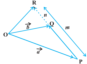
Fig 10.17

Remark If $R$ is the midpoint of $PQ$, then $m=n$. And therefore, from Case I, the midpoint $R$ of $\overrightarrow{{}PQ}$, will have its position vector as

$ \overrightarrow{{}OR}=\frac{\vec{a}+\vec{b}}{2} $

10.6 Product of Two Vectors

So far we have studied about addition and subtraction of vectors. An other algebraic operation which we intend to discuss regarding vectors is their product. We may recall that product of two numbers is a number, product of two matrices is again a matrix. But in case of functions, we may multiply them in two ways, namely, multiplication of two functions pointwise and composition of two functions. Similarly, multiplication of two vectors is also defined in two ways, namely, scalar (or dot) product where the result is a scalar, and vector (or cross) product where the result is a vector. Based upon these two types of products for vectors, they have found various applications in geometry, mechanics and engineering. In this section, we will discuss these two types of products.

10.6.1 Scalar (or dot) product of two vectors

Definition 2 The scalar product of two nonzero vectors $\vec{a}$ and $\vec{b}$, denoted by $\vec{a} \cdot \vec{b}$, is defined as

$ \vec{a} \cdot \vec{b}=|\vec{a}||\vec{b}| \cos \theta $

where, $\theta$ is the angle between $\vec{a}$ and $\vec{b}, 0 \leq \theta \leq \pi$ (Fig 10.19).

If either $\vec{a}=0$ or $\vec{b}=0$ then $\theta$ is not defined, and in this case, we

Fig 10.19 define $\vec{a} \cdot \vec{b}=0$

Observations

1. $\vec{a} \cdot \vec{b}$ is a real number.

2. Let $\vec{a}$ and $\vec{b}$ be two nonzero vectors, then $\vec{a} \cdot \vec{b}=0$ if and only if $\vec{a}$ and $\vec{b}$ are perpendicular to each other. i.e.

$$\vec{a} \cdot \vec{b}=0 \leftrightarrow \vec{a} \perp \vec{b}$$

3. If $\theta=0$, then $\vec{a} \cdot \vec{b}=|\vec{a}||\vec{b}|$

$\quad\quad$ In particular, $\vec{a} \cdot \vec{a}=|\vec{a}|^{2}$, as $\theta$ in this case is 0 .

4. If $\theta=\pi$, then $\vec{a} \cdot \vec{b}=-|\vec{a}||\vec{b}|$

$\quad\quad$In particular, $\vec{a} \cdot \vec{b}=-|\vec{a}||\vec{b}|$, as $\theta$ in this case is $\pi$.

5. In view of the Observations 2 and 3 , for mutually perpendicular unit vectors $\hat{i}, \hat{j}$ and $\hat{k}$, we have

$$ \begin{aligned} & \hat{i} \cdot \hat{i}=\hat{j} \cdot \hat{j}=\hat{k} \cdot \hat{k}=1, \\ & \hat{i} \cdot \hat{j}=\hat{j} \cdot \hat{k}=\hat{k} \cdot \hat{i}=0 \end{aligned} $$

6. The angle between two nonzero vectors $\vec{a}$ and $\vec{b}$ is given by

$$ \cos \theta=\frac{\vec{a} \cdot \vec{b}}{|\vec{a}||\vec{b}|}, \text{ or } \theta=\cos ^{-1}(\frac{\vec{a} \cdot \vec{b}}{|\vec{a}||\vec{b}|}) $$

7. The scalar product is commutative. i.e.

$$ \vec{a} \cdot \vec{b}=\vec{b} \cdot \vec{a} $$

Two important properties of scalar product

Property 1 (Distributivity of scalar product over addition) Let $\vec{a}, \vec{b}$ and $\vec{c}$ be any three vectors, then

$ \vec{a} \cdot(\vec{b}+\vec{c})=\vec{a} \cdot \vec{b}+\vec{a} \cdot \vec{c} $

Property 2 Let $\vec{a}$ and $\vec{b}$ be any two vectors, and 1 be any scalar. Then

$ (\lambda \vec{a}) \cdot \vec{b}=(\lambda \vec{a}) \cdot \vec{b}=\lambda(\vec{a} \cdot \vec{b})=\vec{a} \cdot(\lambda \vec{b}) $

If two vectors $\vec{a}$ and $\vec{b}$ are given in component form as $a_1 \hat{i}+a_2 \hat{j}+a_3 \hat{k}$ and $b_1 \hat{i}+b_2 \hat{j}+b_3 \hat{k}$, then their scalar product is given as

$ \begin{aligned} \vec{a} \cdot \vec{b}= & (a_1 \hat{i}+a_2 \hat{j}+a_3 \hat{k}) \cdot(b_1 \hat{i}+b_2 \hat{j}+b_3 \hat{k}) \\ = & a_1 \hat{i} \cdot(b_1 \hat{i}+b_2 \hat{j}+b_3 \hat{k})+a_2 \hat{j} \cdot(b_1 \hat{i}+b_2 \hat{j}+b_3 \hat{k})+a_3 \hat{k} \cdot(b_1 \hat{i}+b_2 \hat{j}+b_3 \hat{k}) \\ = & a_1 b_1(\hat{i} \cdot \hat{i})+a_1 b_2(\hat{i} \cdot \hat{j})+a_1 b_3(\hat{i} \cdot \hat{k})+a_2 b_1(\hat{j} \cdot \hat{i})+a_2 b_2(\hat{j} \cdot \hat{j})+a_2 b_3(\hat{j} \cdot \hat{k}) \\ & +a_3 b_1(\hat{k} \cdot \hat{i})+a_3 b_2(\hat{k} \cdot \hat{j})+a_3 b_3(\hat{k} \cdot \hat{k}) \text{ (Using the above Properties } 1 \text{ and 2) } \\ = & a_1 b_1+a_2 b_2+a_3 b_3 \\ & \vec{a} \cdot \vec{b}=a_1 b_1+a_2 b_2+a_3 b_3 \end{aligned} $

Thus

10.6.2 Projection of a vector on a line

Suppose a vector $\overrightarrow{{}AB}$ makes an angle $\theta$ with a given directed line $l$ (say), in the anticlockwise direction (Fig 10.20). Then the projection of $\overrightarrow{{}AB}$ on $l$ is a vector $\vec{p}$ (say) with magnitude $|\overrightarrow{{}AB}||\cos \theta|$, and the direction of $\vec{p}$ being the same (or opposite) to that of the line $l$, depending upon whether $\cos \theta$ is positive or negative. The vector $\vec{p}$

Fig 10.20 is called the projection vector, and its magnitude $|\vec{p}|$ is simply called as the projection of the vector $\overrightarrow{{}AB}$ on the directed line $l$.

For example, in each of the following figures (Fig 10.20 (i) to (iv)), projection vector of $\overrightarrow{{}AB}$ along the line $l$ is vector $\overrightarrow{{}AC}$.

Observations

1. If $\hat{p}$ is the unit vector along a line $l$, then the projection of a vector $\vec{a}$ on the line $l$ is given by $\vec{a} \cdot \hat{p}$.

2. Projection of a vector $\vec{a}$ on other vector $\vec{b}$, is given by

$$ \vec{a} \cdot \hat{b}, \quad \text{ or } \quad \vec{a} \cdot(\frac{\vec{b}}{|\vec{b}|}), \text{ or } \frac{1}{|\vec{b}|}(\vec{a} \cdot \vec{b}) $$

3. If $\theta=0$, then the projection vector of $\overrightarrow{{}A B}$ will be $\overrightarrow{{}A B}$ itself and if $\theta=\pi$, then the projection vector of $\overrightarrow{{}AB}$ will be $\overrightarrow{{}BA}$.

4. If $\theta=\frac{\pi}{2}$ or $\theta=\frac{3 \pi}{2}$, then the projection vector of $\overrightarrow{{}A B}$ will be zero vector.

Remark If $\alpha, \beta$ and $\gamma$ are the direction angles of vector $\vec{a}=a_1 \hat{i}+a_2 \hat{j}+a_3 \hat{k}$, then its direction cosines may be given as

$$ \cos \alpha=\frac{\vec{a} \cdot \hat{i}}{|\vec{a}||\hat{i}|}=\frac{a_1}{|\vec{a}|}, \cos \beta=\frac{a_2}{|\vec{a}|}, \text{ and } \cos \gamma=\frac{a_3}{|\vec{a}|} $$

Also, note that $|\vec{a}| \cos \alpha,|\vec{a}| \cos \beta$ and $|\vec{a}| \cos \gamma$ are respectively the projections of $\vec{a}$ along $OX, OY$ and $OZ$. i.e., the scalar components $a_1, a_2$ and $a_3$ of the vector $\vec{a}$, are precisely the projections of $\vec{a}$ along $x$-axis, $y$-axis and $z$-axis, respectively. Further, if $\vec{a}$ is a unit vector, then it may be expressed in terms of its direction cosines as

$$ \vec{a}=\cos \alpha \hat{i}+\cos \beta \hat{j}+\cos \gamma \hat{k} $$

10.6.3 Vector (or cross) product of two vectors

In Section 10.2, we have discussed on the three dimensional right handed rectangular coordinate system. In this system, when the positive $x$-axis is rotated counterclockwise into the positive $y$-axis, a right handed (standard) screw would advance in the direction of the positive $z$-axis (Fig 10.22(i)).

In a right handed coordinate system, the thumb of the right hand points in the direction of the positive $z$-axis when the fingers are curled in the direction away from the positive $x$-axis toward the positive $y$-axis (Fig 10.22(ii)).

Fig 10.22

Definition 3 The vector product of two nonzero vectors $\vec{a}$ and $\vec{b}$, is denoted by $\vec{a} \times \vec{b}$ and defined as

$ \vec{a} \times \vec{b}=|\vec{a} | \vec{b}| \sin \theta \hat{n}, $

where, $\theta$ is the angle between $\vec{a}$ and $\vec{b}, 0 \leq \theta \leq \pi$ and $\hat{n}$ is a unit vector perpendicular to both $\vec{a}$ and $\vec{b}$, such that $\vec{a}, \vec{b}$ and $\hat{n}$ form a right handed system (Fig 10.23). i.e., the $-\hat{\boldsymbol{{}n}}$

right handed system rotated from $\vec{a}$ to $\vec{b}$ moves in the direction of $\hat{n}$.

Fig 10.23

If either $\vec{a}=\overrightarrow{{}0}$ or $\vec{b}=\overrightarrow{{}0}$, then $\theta$ is not defined and in this case, we define $\vec{a} \times \vec{b}=\overrightarrow{{}0}$.

Observations

1. $\vec{a} \times \vec{b}$ is a vector.

2. Let $\vec{a}$ and $\vec{b}$ be two nonzero vectors. Then $\vec{a} \times \vec{b}=\overrightarrow{{}0}$ if and only if $\vec{a}$ and $\vec{b}$ are parallel (or collinear) to each other, i.e.,

$ \vec{a} \times \vec{b}=\overrightarrow{{}0} \leftrightarrow \vec{a} | \vec{b} $

In particular, $\vec{a} \times \vec{a}=\overrightarrow{{}0}$ and $\vec{a} \times(-\vec{a})=\overrightarrow{{}0}$, since in the first situation, $\theta=0$ and in the second one, $\theta=\pi$, making the value of $\sin \theta$ to be 0 .

3. If $\theta=\frac{\pi}{2}$ then $\vec{a} \times \vec{b}=|\vec{a}||\vec{b}|$.

4. In view of the Observations 2 and 3 , for mutually perpendicular unit vectors $\hat{i}, \hat{j}$ and $\hat{k}$ (Fig 10.24), we have

$ \begin{aligned} & \hat{i} \times \hat{i}=\hat{j} \times \hat{j}=\hat{k} \times \hat{k}=\overrightarrow{{}0} \\ & \hat{i} \times \hat{j}=\hat{k}, \quad \hat{j} \times \hat{k}=\hat{i}, \quad \hat{k} \times \hat{i}=\hat{j} \end{aligned} $

Fig 10.24

5. In terms of vector product, the angle between two vectors $\vec{a}$ and $\vec{b}$ may be given as

$$ \sin \theta=\frac{|\vec{a} \times \vec{b}|}{|\vec{a} | \vec{b}|} $$

6. It is always true that the vector product is not commutative, as $ \vec{a} \times \vec{b} =-\vec{b} \times \vec{a}$. Indeed, $ \vec{a} \times \vec{b}=|\vec{a}||\vec{b}| \sin \theta \hat{n}$, where $ \vec{a}, \vec{b} $ and $ \hat{n} $ form a right handed system, i.e., $\theta$ is traversed from $\vec{a} $ to $\vec{b} $ , Fig 10.25

Fig 10.25 (i)(ii)

Thus, if we assume $\vec{a}$ and $ \vec {b} $ to lie in the plane of the paper, then $ \hat{n} $ and $ \hat {n} _ {1} $ both will be perpendicular to the plane of the paper. But, $ \hat{n} $ being directed above the paper while $ \hat {n} _ {1} $ directed below the paper. i.e. $ \hat {n} _ {1} =-\hat {n} $.

Hence $$ \begin{aligned} \vec{a} \times \vec{b} & =|\vec{a} | \vec{b}| \sin \hat{n} \\ & =-|\vec{a} | \vec{b}| \sin \theta \hat{n}_1=-\vec{b} \times \vec{a} \end{aligned} $$

7. In view of the Observations 4 and 6 , we have

$$ \hat{j} \times \hat{i}=-\hat{k}, \quad \hat{k} \times \hat{j}=-\hat{i} \text{ and } \hat{i} \times \hat{k}=-\hat{j} \text{. } $$

8. If $\vec{a}$ and $\vec{b}$ represent the adjacent sides of a triangle then its area is given as $\frac{1}{2}|\vec{a} \times \vec{b}|$.

By definition of the area of a triangle, we have from Fig 10.26,

Area of triangle $ABC=\frac{1}{2} AB \cdot CD$.

Fig 10.26

But $AB=|\vec{b}|$ (as given), and $CD=|\vec{a}| \sin \theta$.

Thus, Area of triangle $ABC=\frac{1}{2}|\vec{b}||\vec{a}| \sin \theta=\frac{1}{2}|\vec{a} \times \vec{b}|$.

9. If $\vec{a}$ and $\vec{b}$ represent the adjacent sides of a parallelogram, then its area is given by $|\vec{a} \times \vec{b}|$.

From Fig 10.27, we have

Area of parallelogram $ABCD=AB$. $DE$.

But $AB=|\vec{b}|$ (as given), and

$DE=|\vec{a}| \sin \theta$.

Thus,

Fig 10.27

Area of parallelogram $ABCD=|\vec{b} | \vec{a}| \sin \theta=|\vec{a} \times \vec{b}|$.

We now state two important properties of vector product.

Property 3 (Distributivity of vector product over addition): If $\vec{a}, \vec{b}$ and $\vec{c}$ are any three vectors and $\lambda$ be a scalar, then

(i) $\vec{a} \times(\vec{b}+\vec{c})=\vec{a} \times \vec{b}+\vec{a} \times \vec{c}$

(ii) $\lambda(\vec{a} \times \vec{b})=(\lambda \vec{a}) \times \vec{b}=\vec{a} \times(\lambda \vec{b})$

Let $\vec{a}$ and $\vec{b}$ be two vectors given in component form as $a_1 \hat{i}+a_2 \hat{j}+a_3 \hat{k}$ and $b_1 \hat{i}+b_2 \hat{j}+b_3 \hat{k}$, respectively. Then their cross product may be given by

$$ \vec{a} \times \vec{b}= \begin{vmatrix} \hat{i} & \hat{j} & \hat{k} \\ a_1 & a_2 & a_3 \\ b_1 & b_2 & b_3 \end{vmatrix} $$

Explanation We have

$$ \begin{aligned} \vec{a} \times \vec{b}= & (a_1 \hat{i}+a_2 \hat{j}+a_3 \hat{k}) \times(b_1 \hat{i}+b_2 \hat{j}+b_3 \hat{k}) \\ = & a_1 b_1(\hat{i} \times \hat{i})+a_1 b_2(\hat{i} \times \hat{j})+a_1 b_3(\hat{i} \times \hat{k})+a_2 b_1(\hat{j} \times \hat{i}) \\ & +a_2 b_2(\hat{j} \times \hat{j})+a_2 b_3(\hat{j} \times \hat{k}) \\ & +a_3 b_1(\hat{k} \times \hat{i})+a_3 b_2(\hat{k} \times \hat{j})+a_3 b_3(\hat{k} \times \hat{k}) \\ = & a_1 b_2(\hat{i} \times \hat{j})-a_1 b_3(\hat{k} \times \hat{i})-a_2 b_1(\hat{i} \times \hat{j}) \\ & +a_2 b_3(\hat{j} \times \hat{k})+a_3 b_1(\hat{k} \times \hat{i})-a_3 b_2(\hat{j} \times \hat{k}) \end{aligned} $$

(by Property 1)

(as $\hat{i} \times \hat{i}=\hat{j} \times \hat{j}=\hat{k} \times \hat{k}=0$ and $\hat{i} \times \hat{k}=-\hat{k} \times \hat{i}, \hat{j} \times \hat{i}=-\hat{i} \times \hat{j}$ and $\hat{k} \times \hat{j}=-\hat{j} \times \hat{k}$ )

$$ \begin{aligned} = & a_1 b_2 \hat{k}-a_1 b_3 \hat{j}-a_2 b_1 \hat{k}+a_2 b_3 \hat{i}+a_3 b_1 \hat{j}-a_3 b_2 \hat{i} \\ & (\text{ as } \hat{i} \times \hat{j}=\hat{k}, \hat{j} \times \hat{k}=\hat{i} \text{ and } \hat{k} \times \hat{i}=\hat{j}) \\ = & (a_2 b_3-a_3 b_2) \hat{i}-(a_1 b_3-a_3 b_1) \hat{j}+(a_1 b_2-a_2 b_1) \hat{k} \\ = & \begin{vmatrix} \hat{i} & \hat{j} & \hat{k} \\ a_1 & a_2 & a_3 \\ b_1 & b_2 & b_3 \end{vmatrix} \end{aligned} $$

Summary

Position vector of a point $P(x, y, z)$ is given as $\overrightarrow{{}OP}(=\vec{r})=x \hat{i}+y \hat{j}+z \hat{k}$, and its magnitude by $\sqrt{x^{2}+y^{2}+z^{2}}$.

The scalar components of a vector are its direction ratios, and represent its projections along the respective axes.

The magnitude $(r)$, direction ratios $(a, b, c)$ and direction cosines $(l, m, n)$ of any vector are related as:

$ l=\frac{a}{r}, \quad m=\frac{b}{r}, \quad n=\frac{c}{r} $

The vector sum of the three sides of a triangle taken in order is $\overrightarrow{{}0}$.

• The vector sum of two coinitial vectors is given by the diagonal of the parallelogram whose adjacent sides are the given vectors.
• The multiplication of a given vector by a scalar $\lambda$, changes the magnitude of the vector by the multiple $|\lambda|$, and keeps the direction same (or makes it opposite) according as the value of $\lambda$ is positive (or negative).

For a given vector $\vec{a}$, the vector $\hat{a}=\frac{\vec{a}}{|\vec{a}|}$ gives the unit vector in the direction of $\vec{a}$.

• The position vector of a point $R$ dividing a line segment joining the points $P$ and $Q$ whose position vectors are $\vec{a}$ and $\vec{b}$ respectively, in the ratio $m: n$

(i) internally, is given by $\frac{n \vec{a}+m \vec{b}}{m+n}$.

(ii) externally, is given by $\frac{m \vec{b}-n \vec{a}}{m-n}$.

• The scalar product of two given vectors $\vec{a}$ and $\vec{b}$ having angle $\theta$ between them is defined as

$$ \vec{a} \cdot \vec{b}=|\vec{a}||\vec{b}| \cos \theta $$

Also, when $\vec{a} \cdot \vec{b}$ is given, the angle ’ $\theta$ ’ between the vectors $\vec{a}$ and $\vec{b}$ may be determined by

$$ \cos \theta=\frac{\vec{a} \cdot \vec{b}}{|\vec{a}||\vec{b}|} $$

$\Delta$ If $\theta$ is the angle between two vectors $\vec{a}$ and $\vec{b}$, then their cross product is given as

$$ \vec{a} \times \vec{b}=|\vec{a} | \vec{b}| \sin \theta \hat{n} $$

where $\hat{n}$ is a unit vector perpendicular to the plane containing $\vec{a}$ and $\vec{b}$. Such that $\vec{a}, \vec{b}, \hat{n}$ form right handed system of coordinate axes.

• If we have two vectors $\vec{a}$ and $\vec{b}$, given in component form as $\vec{a}=a _ {1} \hat{i}+a _ {2} \hat{j}+a _ {3} \hat{k}$ and $\vec{b}=b _ {1} \hat{i}+b _ {2} \hat{j}+b _ {3} \hat{k}$ and $\lambda$ any scalar, then

$$ \begin{aligned} \vec{a}+\vec{b} & =(a _ {1}+b _ {1}) \hat{i}+(a _ {2}+b _ {2}) \hat{j}+(a _ {3}+b _ {3}) \hat{k} \\ \lambda \vec{a} & =(\lambda a _ {1}) \hat{i}+(\lambda a _ {2}) \hat{j}+(\lambda a _ {3}) \hat{k} \\ \vec{a} \cdot \vec{b} & =a _ {1} b _ {1}+a _ {2} b _ {2}+a _ {3} b _ {3} \end{aligned} $$

$$ \text{ and } \quad \vec{a} \times \vec{b}= \begin{vmatrix} \hat{i} & \hat{j} & \hat{k} \\ a_1 & b_1 & c_1 \\ a_2 & b_2 & c_2 \end{vmatrix} \text{. } $$

Historical Note

The word vector has been derived from a Latin word vectus, which means “to carry”. The germinal ideas of modern vector theory date from around 1800 when Caspar Wessel (1745-1818) and Jean Robert Argand (1768-1822) described that how a complex number $a+i b$ could be given a geometric interpretation with the help of a directed line segment in a coordinate plane. William Rowen Hamilton (1805-1865) an Irish mathematician was the first to use the term vector for a directed line segment in his book Lectures on Quaternions (1853). Hamilton’s method of quaternions (an ordered set of four real numbers given as: $a+b \hat{i}+c \hat{j}+d \hat{k}, \hat{i}, \hat{j}, \hat{k}$ following certain algebraic rules) was a solution to the problem of multiplying vectors in three dimensional space. Though, we must mention here that in practice, the idea of vector concept and their addition was known much earlier ever since the time of Aristotle (384-322 B.C.), a Greek philosopher, and pupil of Plato (427-348 B.C.). That time it was supposed to be known that the combined action of two or more forces could be seen by adding them according to parallelogram law. The correct law for the composition of forces, that forces add vectorially, had been discovered in the case of perpendicular forces by Stevin-Simon (1548-1620). In 1586 A.D., he analysed the principle of geometric addition of forces in his treatise DeBeghinselen der Weeghconst (“Principles of the Art of Weighing”), which caused a major breakthrough in the development of mechanics. But it took another 200 years for the general concept of vectors to form.

In the 1880, Josaih Willard Gibbs (1839-1903), an American physicist and mathematician, and Oliver Heaviside (1850-1925), an English engineer, created what we now know as vector analysis, essentially by separating the real (scalar) part of quaternion from its imaginary (vector) part. In 1881 and 1884, Gibbs printed a treatise entitled Element of Vector Analysis. This book gave a systematic and concise account of vectors. However, much of the credit for demonstrating the applications of vectors is due to the D. Heaviside and P.G. Tait (1831-1901) who contributed significantly to this subject.