Chapter-12 Linear Programming
The mathematical experience of the student is incomplete if he never had the opportunity to solve a problem invented by himself. - G. POLYA
12.1 Introduction
In earlier classes, we have discussed systems of linear equations and their applications in day to day problems. In Class XI, we have studied linear inequalities and systems of linear inequalities in two variables and their solutions by graphical method. Many applications in mathematics involve systems of inequalities/equations. In this chapter, we shall apply the systems of linear inequalities/equations to solve some real life problems of the type as given below:
A furniture dealer deals in only two items-tables and chairs. He has Rs 50,000 to invest and has storage space of at most 60 pieces. A table costs Rs 2500 and a chair Rs 500 . He estimates that from the sale of one table, he can make a profit of Rs 250 and that from the sale of one

L. Kantorovich chair a profit of Rs 75 . He wants to know how many tables and chairs he should buy from the available money so as to maximise his total profit, assuming that he can sell all the items which he buys.Such type of problems which seek to maximise (or, minimise) profit (or, cost) form a general class of problems called optimisation problems. Thus, an optimisation problem may involve finding maximum profit, minimum cost, or minimum use of resources etc.
A special but a very important class of optimisation problems is linear programming problem. The above stated optimisation problem is an example of linear programming problem. Linear programming problems are of much interest because of their wide applicability in industry, commerce, management science etc.
In this chapter, we shall study some linear programming problems and their solutions by graphical method only, though there are many other methods also to solve such problems.
12.2 Linear Programming Problem and its Mathematical Formulation
We begin our discussion with the above example of furniture dealer which will further lead to a mathematical formulation of the problem in two variables. In this example, we observe
(i) The dealer can invest his money in buying tables or chairs or combination thereof. Further he would earn different profits by following different investment strategies.
(ii) There are certain overriding conditions or constraints viz., his investment is limited to a maximum of Rs 50,000 and so is his storage space which is for a maximum of 60 pieces.
Suppose he decides to buy tables only and no chairs, so he can buy $50000 \div 2500$, i.e., 20 tables. His profit in this case will be Rs $(250 \times 20)$, i.e., Rs $\mathbf{5 0 0 0}$.
Suppose he chooses to buy chairs only and no tables. With his capital of Rs 50,000, he can buy $50000 \div 500$, i.e. 100 chairs. But he can store only 60 pieces. Therefore, he is forced to buy only 60 chairs which will give him a total profit of Rs $(60 \times 75)$, i.e., Rs 4500.
There are many other possibilities, for instance, he may choose to buy 10 tables and 50 chairs, as he can store only 60 pieces. Total profit in this case would be Rs $(10 \times 250+50 \times 75)$, i.e., Rs $\mathbf{6 2 5 0}$ and so on.
We, thus, find that the dealer can invest his money in different ways and he would earn different profits by following different investment strategies.
Now the problem is: How should he invest his money in order to get maximum profit? To answer this question, let us try to formulate the problem mathematically.
12.2.1 Mathematical formulation of the problem
Let $x$ be the number of tables and $y$ be the number of chairs that the dealer buys. Obviously, $x$ and $y$ must be non-negative, i.e.,
$$ \begin{align*} & x \geq 0 \tag{1}\\ & y \geq 0 \tag{2} \end{align*} \text { (Non-negative constraints) } $$
The dealer is constrained by the maximum amount he can invest (Here it is Rs 50,000 ) and by the maximum number of items he can store (Here it is 60).
Stated mathematically,
or $$ \begin{array}{rlrl} 2500 x+500 y & \leq 50,000 & \text { (investment constraint ) } \\ 5 x+y & \leq 100 & & \\ x+y & \leq 60 & & \text { (storage constraint) } \tag{4} \end{array} $$
The dealer wants to invest in such a way so as to maximise his profit, say, $Z$ which stated as a function of $x$ and $y$ is given by
$Z=250 x+75 y$ (called objective function)
Mathematically, the given problems now reduces to:
Maximise $Z=250 x+75 y$
subject to the constraints:
$$ \begin{aligned} 5 x+y & \leq 100 \\ x+y & \leq 60 \\ x \geq 0, y & \geq 0 \end{aligned} $$
So, we have to maximise the linear function $Z$ subject to certain conditions determined by a set of linear inequalities with variables as non-negative. There are also some other problems where we have to minimise a linear function subject to certain conditions determined by a set of linear inequalities with variables as non-negative. Such problems are called Linear Programming Problems.
Thus, a Linear Programming Problem is one that is concerned with finding the optimal value (maximum or minimum value) of a linear function (called objective function) of several variables (say $x$ and $y$ ), subject to the conditions that the variables are non-negative and satisfy a set of linear inequalities (called linear constraints). The term linear implies that all the mathematical relations used in the problem are linear relations while the term programming refers to the method of determining a particular programme or plan of action.
Before we proceed further, we now formally define some terms (which have been used above) which we shall be using in the linear programming problems:
Objective function Linear function $Z=a x+b y$, where $a, b$ are constants, which has to be maximised or minimized is called a linear objective function.
In the above example, $Z=250 x+75 y$ is a linear objective function. Variables $x$ and $y$ are called decision variables.
Constraints The linear inequalities or equations or restrictions on the variables of a linear programming problem are called constraints. The conditions $x \geq 0, y \geq 0$ are called non-negative restrictions. In the above example, the set of inequalities (1) to (4) are constraints.
Optimisation problem A problem which seeks to maximise or minimise a linear function (say of two variables $x$ and $y$ ) subject to certain constraints as determined by a set of linear inequalities is called an optimisation problem. Linear programming problems are special type of optimisation problems. The above problem of investing a given sum by the dealer in purchasing chairs and tables is an example of an optimisation problem as well as of a linear programming problem.
We will now discuss how to find solutions to a linear programming problem. In this chapter, we will be concerned only with the graphical method.
12.2.2 Graphical method of solving linear programming problems
In Class XI, we have learnt how to graph a system of linear inequalities involving two variables $x$ and $y$ and to find its solutions graphically. Let us refer to the problem of investment in tables and chairs discussed in Section 12.2. We will now solve this problem graphically. Let us graph the constraints stated as linear inequalities:
$$ \begin{align*} 5 x+y & \leq 100 \tag{1} \\ x+y & \leq 60 \tag{2} \\ x & \geq 0 \tag{3} \\ y & \geq 0 \tag{4} \end{align*} $$
The graph of this system (shaded region) consists of the points common to all half planes determined by the inequalities (1) to (4) (Fig 12.1). Each point in this region represents a feasible choice open to the dealer for investing in tables and chairs. The region, therefore, is called the feasible region for the problem. Every point of this region is called a feasible solution to the problem. Thus, we have,
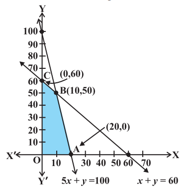
Fig 12.1
Feasible region The common region determined by all the constraints including non-negative constraints $x, y \geq 0$ of a linear programming problem is called the feasible region (or solution region) for the problem. In Fig 12.1, the region OABC (shaded) is the feasible region for the problem. The region other than feasible region is called an infeasible region.
Feasible solutions Points within and on the boundary of the feasible region represent feasible solutions of the constraints. In Fig 12.1, every point within and on the boundary of the feasible region $OABC$ represents feasible solution to the problem. For example, the point $(10,50)$ is a feasible solution of the problem and so are the points $(0,60),(20,0)$ etc.
Any point outside the feasible region is called an infeasible solution. For example, the point $(25,40)$ is an infeasible solution of the problem.
Optimal (feasible) solution: Any point in the feasible region that gives the optimal value (maximum or minimum) of the objective function is called an optimal solution.
Now, we see that every point in the feasible region $OABC$ satisfies all the constraints as given in (1) to (4), and since there are infinitely many points, it is not evident how we should go about finding a point that gives a maximum value of the objective function $Z=250 x+75 y$. To handle this situation, we use the following theorems which are fundamental in solving linear programming problems. The proofs of these theorems are beyond the scope of the book.
Theorem 1 Let $R$ be the feasible region (convex polygon) for a linear programming problem and let $Z=a x+b y$ be the objective function. When $Z$ has an optimal value (maximum or minimum), where the variables $x$ and $y$ are subject to constraints described by linear inequalities, this optimal value must occur at a corner point* (vertex) of the feasible region.
Theorem 2 Let $R$ be the feasible region for a linear programming problem, and let $Z=a x+b y$ be the objective function. If $R$ is bounded**, then the objective function $Z$ has both a maximum and a minimum value on $R$ and each of these occurs at a corner point (vertex) of R.
Remark If $R$ is unbounded, then a maximum or a minimum value of the objective function may not exist. However, if it exists, it must occur at a corner point of R. (By Theorem 1).
In the above example, the corner points (vertices) of the bounded (feasible) region are: $O, A, B$ and $C$ and it is easy to find their coordinates as $(0,0),(20,0),(10,50)$ and $(0,60)$ respectively. Let us now compute the values of $Z$ at these points.
We have
| Vertex of the Feasible region | Correasponding calue of Z (in Rs) |
|---|---|
| O(0,0) | 0 |
| C(0,60) | 4500 |
| B(10,50) | $ \mathbf{6 2 5 0} $ |
| A(20,0) | 5000 |
-
A corner point of a feasible region is a point in the region which is the intersection of two boundary lines.
-
A feasible region of a system of linear inequalities is said to be bounded if it can be enclosed within a circle. Otherwise, it is called unbounded. Unbounded means that the feasible region does extend indefinitely in any direction.
We observe that the maximum profit to the dealer results from the investment strategy $(10,50)$, i.e. buying 10 tables and 50 chairs.
This method of solving linear programming problem is referred as Corner Point Method. The method comprises of the following steps:
1. Find the feasible region of the linear programming problem and determine its corner points (vertices) either by inspection or by solving the two equations of the lines intersecting at that point.
2. Evaluate the objective function $Z=a x+b y$ at each corner point. Let $\mathbf{M}$ and $m$, respectively denote the largest and smallest values of these points.
3. (i) When the feasible region is bounded, $M$ and $m$ are the maximum and minimum values of $Z$.
(ii) In case, the feasible region is unbounded, we have:
4. (a) $M$ is the maximum value of $Z$, if the open half plane determined by $a x+b y>M$ has no point in common with the feasible region. Otherwise, $Z$ has no maximum value.
(b) Similarly, $m$ is the minimum value of $Z$, if the open half plane determined by $a x+b y<m$ has no point in common with the feasible region. Otherwise, $Z$ has no minimum value.
We will now illustrate these steps of Corner Point Method by considering some examples:
Example 1 Solve the following linear programming problem graphically:
Maximise $Z=4 x+y$ subject to the constraints:
$$ \begin{aligned} x+y & \leq 50 \\ 3 x+y & \leq 90 \\ x \geq 0, y & \geq 0 \end{aligned} $$
Solution The shaded region in Fig 12.2 is the feasible region determined by the system of constraints (2) to (4). We observe that the feasible region OABC is bounded. So, we now use Corner Point Method to determine the maximum value of $Z$.
The coordinates of the corner points $O, A, B$ and $C$ are $(0,0),(30,0),(20,30)$ and $(0,50)$ respectively. Now we evaluate $Z$ at each corner point.
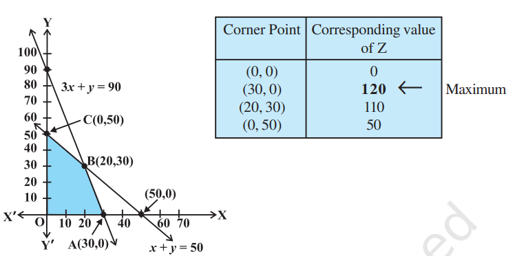
Fig 12.2
Hence, maximum value of $Z$ is 120 at the point $(30,0)$.
Example 2 Solve the following linear programming problem graphically:
Minimise $Z=200 x+500 y$
subject to the constraints:
$$ \begin{align*} x+2 y & \geq 10 \tag{1}\\ 3 x+4 y & \leq 24 \tag{2}\\ x \geq 0, y & \geq 0 \tag{3} \end{align*} $$
Solution The shaded region in Fig 12.3 is the feasible region ABC determined by the system of constraints (2) to (4), which is bounded. The coordinates of corner points A, B and $C$ are $(0,5),(4,3)$ and $(0,6)$ respectively. Now we evaluate $Z=200 x+500 y$ at these points.
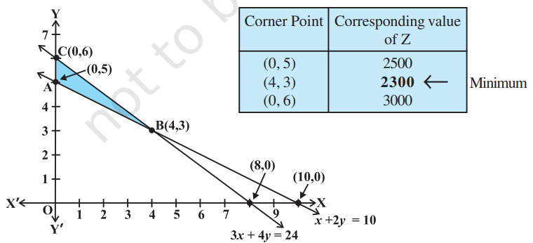
Fig 12.3
Hence, minimum value of $Z$ is 2300 attained at the point $(4,3)$
Example 3 Solve the following problem graphically:
Minimise and Maximise $Z=3 x+9 y$
subject to the constraints: $\quad x+3 y \leq 60$
$$ \begin{align*} x+3 y & \leq 60 \tag{1}\\ x+y & \geq 10 \tag{2}\\ x & \leq y \tag{3}\\ x \geq 0, y & \geq 0 \tag{4} \end{align*} $$
Solution First of all, let us graph the feasible region of the system of linear inequalities (2) to (5). The feasible region $ABCD$ is shown in the Fig 12.4. Note that the region is bounded. The coordinates of the corner points A, B, C and D are $(0,10),(5,5),(15,15)$ and $(0,20)$ respectively.
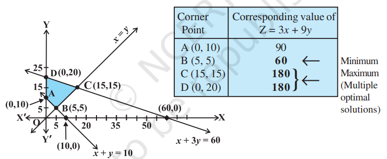
Fig 12.4
We now find the minimum and maximum value of $Z$. From the table, we find that the minimum value of $Z$ is 60 at the point $B(5,5)$ of the feasible region.
The maximum value of $Z$ on the feasible region occurs at the two corner points $C(15,15)$ and $D(0,20)$ and it is 180 in each case.
Remark Observe that in the above example, the problem has multiple optimal solutions at the corner points $C$ and $D$, i.e. the both points produce same maximum value 180 . In such cases, you can see that every point on the line segment CD joining the two corner points $C$ and $D$ also give the same maximum value. Same is also true in the case if the two points produce same minimum value.
Example 4 Determine graphically the minimum value of the objective function
$$ Z=-50 x+20 y $$
subject to the constraints:
$$ \begin{aligned} & 2 x-y \geq-5 \\ & 3 x+y \geq 3 \\ & 2 x-3 y \leq 12 \\ & x \geq 0, y \geq 0 \end{aligned} $$
Solution First of all, let us graph the feasible region of the system of inequalities (2) to (5). The feasible region (shaded) is shown in the Fig 12.5. Observe that the feasible region is unbounded.
We now evaluate $Z$ at the corner points.
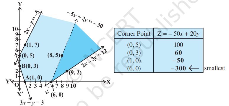
Fig 12.5
From this table, we find that -300 is the smallest value of $Z$ at the corner point $(6,0)$. Can we say that minimum value of $Z$ is -300 ? Note that if the region would have been bounded, this smallest value of $Z$ is the minimum value of $Z$ (Theorem 2). But here we see that the feasible region is unbounded. Therefore, -300 may or may not be the minimum value of $Z$. To decide this issue, we graph the inequality
$$ -50 x+20 y<-300 \text{ (see Step 3(ii) of corner Point Method.) } $$
i.e., $$ -5 x+2 y<-30 $$
and check whether the resulting open half plane has points in common with feasible region or not. If it has common points, then -300 will not be the minimum value of $Z$. Otherwise, -300 will be the minimum value of $Z$.
As shown in the Fig 12.5, it has common points. Therefore, $Z=-50 x+20 y$ has no minimum value subject to the given constraints.
In the above example, can you say whether $z=-50 x+20 y$ has the maximum value 100 at $(0,5)$ ? For this, check whether the graph of $-50 x+20 y>100$ has points in common with the feasible region. (Why?)
Example 5 Minimise $Z=3 x+2 y$
subject to the constraints:
$$ \begin{align*} x+y & \geq 8 \tag{1}\\ 3 x+5 y & \leq 15 \tag{2}\\ x \geq 0, y & \geq 0 \tag{3} \end{align*} $$
Solution Let us graph the inequalities (1) to (3) (Fig 12.6). Is there any feasible region? Why is so?
From Fig 12.6, you can see that there is no point satisfying all the constraints simultaneously. Thus, the problem is having no feasible region and hence no feasible solution.
Remarks From the examples which we have discussed so far, we notice some general features of linear programming problems:
(i) The feasible region is always a convex region.
(ii) The maximum (or minimum)
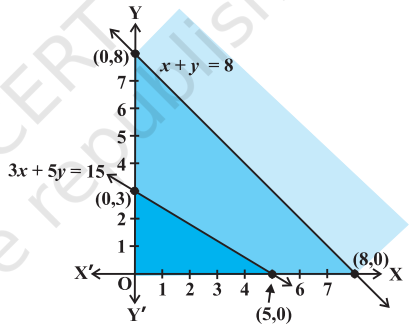
Fig 12.6 solution of the objective function occurs at the vertex (corner) of the feasible region. If two corner points produce the same maximum (or minimum) value of the objective function, then every point on the line segment joining these points will also give the same maximum (or minimum) value.
EXERCISE 12.1
Solve the following Linear Programming Problems graphically:
1. Maximise $Z=3 x+4 y$
subject to the constraints : $x+y \leq 4, x \geq 0, y \geq 0$.
Show Answer
Solution
The feasible region determined by the constraints, $x+y \leq 4, x \geq 0, y \geq 0$, is as follows.

The corner points of the feasible region are $O(0,0), A(4,0)$, and $B(0,4)$. The values of $Z$ at these points are as follows.
| Corner point | $\mathbf{Z}=\mathbf{3 x}+\mathbf{4} \boldsymbol{{}y}$ | |
|---|---|---|
| $O(0,0)$ | 0 | |
| $A(4,0)$ | 12 | |
| $B(0,4)$ | 16 | $\longleftarrow$ Maximum |
Therefore, the maximum value of $Z$ is 16 at the point $B(0,4)$.
2. Minimise $Z=-3 x+4 y$
subject to $x+2 y \leq 8,3 x+2 y \leq 12, x \geq 0, y \geq 0$.
Show Answer
Solution
The feasible region determined by the system of constraints, $x+2 y \leq 8,3 x+2 y \leq 12, x \geq$ 0 , and $y \geq 0$, is as follows.

The corner points of the feasible region are $O(0,0), A(4,0), B(2,3)$, and $C(0,4)$. The values of $Z$ at these corner points are as follows.
| Corner point | $\mathbf{Z}=\mathbf{- 3 x + 4 y}$ | |
|---|---|---|
| $0(0,0)$ | 0 | |
| $A(4,0)$ | -12 | $\longleftarrow$ Minimum |
| $B(2,3)$ | 6 | |
| $C(0,4)$ | 16 |
Therefore, the minimum value of $Z$ is -12 at the point $(4,0)$.
3. Maximise $Z=5 x+3 y$
subject to $3 x+5 y \leq 15,5 x+2 y \leq 10, x \geq 0, y \geq 0$.
Show Answer
Solution
The feasible region determined by the system of constraints, $3 x+5 y \leq 15$, $5 x+2 y \leq 10, x \geq 0$, and $y \geq 0$, are as follows.

The corner points of the feasible region are $O(0,0), A(2,0), B(0,3)$, and $C(\frac{20}{19}, \frac{45}{19})$. The values of $Z$ at these corner points are as follows.
| Corner point | $\mathbf{Z}=\mathbf{5} \boldsymbol{{}x}+\mathbf{3} \boldsymbol{{}y}$ | |
|---|---|---|
| $O(0,0)$ | 0 | |
| $A(2,0)$ | 10 | |
| $B(0,3)$ | 9 | |
| $C(\frac{20}{19}, \frac{45}{19})$ | $\frac{235}{19}$ | $\longleftarrow$ Maximum |
4. Minimise $Z=3 x+5 y$
such that $x+3 y \geq 3, x+y \geq 2, x, y \geq 0$.
Show Answer
Solution
The feasible region determined by the system of constraints, $x+3 y \geq 3, x+y \geq 2$, and $x$, $y \geq 0$, is as follows.

It can be seen that the feasible region is unbounded.
The corner points of the feasible region are $A(3,0), B(\frac{3}{2}, \frac{1}{2})$, and $C(0,2)$.
The values of $Z$ at these corner points are as follows.
| Corner point | $\mathbf{Z}=\mathbf{3} \boldsymbol{{}x}+\mathbf{5} \boldsymbol{{}y}$ | |
|---|---|---|
| $A(3,0)$ | 9 | |
| $B(\frac{3}{2}, \frac{1}{2})$ | 7 | $\longleftarrow$Smallest |
| $C(0,2)$ | 10 |
As the feasible region is unbounded, therefore, 7 may or may not be the minimum value of $Z$.
For this, we draw the graph of the inequality, $3 x+5 y<7$, and check whether the resulting half plane has points in common with the feasible region or not.
It can be seen that the feasible region has no common point with $3 x+5 y<7$ Therefore,
the minimum value of $Z$ is 7 at $(\frac{3}{2}, \frac{1}{2})$.
5. Maximise $Z=3 x+2 y$
subject to $x+2 y \leq 10,3 x+y \leq 15, x, y \geq 0$.
Show Answer
Solution
The feasible region determined by the constraints, $x+2 y \leq 10,3 x+y \leq 15, x \geq 0$, and $y \geq 0$, is as follows.

The corner points of the feasible region are $A(5,0), B(4,3)$, and $C(0,5)$.
The values of $Z$ at these corner points are as follows.
| Corner point | $\mathbf{Z}=\mathbf{3 x}+\mathbf{2} \boldsymbol{{}y}$ | |
|---|---|---|
| $A(5,0)$ | 15 | |
| $B(4,3)$ | 18 | $\longleftarrow$ Maximum |
| $C(0,5)$ | 10 |
Therefore, the maximum value of $Z$ is 18 at the point $(4,3)$.
6. Minimise $Z=x+2 y$
subject to $2 x+y \geq 3, x+2 y \geq 6, x, y \geq 0$.
Show that the minimum of $Z$ occurs at more than two points.
Show Answer
Solution
The feasible region determined by the constraints, $2 x+y \geq 3, x+2 y \geq 6, x \geq 0$, and $y$ $\geq 0$, is as follows.

The corner points of the feasible region are $A(6,0)$ and $B(0,3)$.
The values of $Z$ at these corner points are as follows.
| Corner point | $Z=x+2 y$ |
|---|---|
| $A(6,0)$ | 6 |
| $B(0,3)$ | 6 |
It can be seen that the value of $Z$ at points $A$ and $B$ is same. If we take any other point such as $(2,2)$ on line $x+2 y=6$, then $Z=6$
Thus, the minimum value of $Z$ occurs for more than 2 points.
Therefore, the value of $Z$ is minimum at every point on the line, $x+2 y=6$
7. Minimise and Maximise $Z=5 x+10 y$
subject to $x+2 y \leq 120, x+y \geq 60, x-2 y \geq 0, x, y \geq 0$.
Show Answer
Solution
The feasible region determined by the constraints, $x+2 y \leq 120, x+y \geq 60, x-2 y \geq$ $0, x \geq 0$, and $y \geq 0$, is as follows.

The corner points of the feasible region are $A(60,0), B(120,0), C(60,30)$, and $D(40$, 20).
The values of $Z$ at these corner points are as follows.
| Corner point | $\mathbf{Z}=\mathbf{5} \boldsymbol{{}x}+\mathbf{1 0} \boldsymbol{{}y}$ | |
|---|---|---|
| $A(60,0)$ | 300 | $\longleftarrow$ Minimum |
| $B(120,0)$ | 600 | $\longleftarrow$ Maximum |
| $C(60,30)$ | 600 | $\longleftarrow$ Maximum |
| $D(40,20)$ | 400 |
The minimum value of $Z$ is 300 at $(60,0)$ and the maximum value of $Z$ is 600 at all the points on the line segment joining $(120,0)$ and $(60,30)$.
8. Minimise and Maximise $Z=x+2 y$
subject to $x+2 y \geq 100,2 x-y \leq 0,2 x+y \leq 200 ; x, y \geq 0$.
Show Answer
Solution
The feasible region determined by the constraints, $x+2 y \geq 100,2 x-y \leq 0,2 x+y \leq$ $200, x \geq 0$, and $y \geq 0$, is as follows.

The corner points of the feasible region are $A(0,50), B(20,40), C(50,100)$, and $D(0$, 200).
The values of $Z$ at these corner points are as follows.
| Corner point | $\mathbf{Z}=\boldsymbol{{}x}+\mathbf{2} \boldsymbol{{}y}$ | |
|---|---|---|
| $A(0,50)$ | 100 | $\longleftarrow$ Minimum |
| $B(20,40)$ | 100 | $\longleftarrow$ Minimum |
| $C(50,100)$ | 250 | |
| $D(0,200)$ | 400 | $\longleftarrow$ Maximum |
The maximum value of $Z$ is 400 at $(0,200)$ and the minimum value of $Z$ is 100 at all the points on the line segment joining the points $(0,50)$ and $(20,40)$.
9. Maximise $Z=-x+2 y$, subject to the constraints:
$$x \geq 3, x+y \geq 5, x+2 y \geq 6, y \geq 0$$
Show Answer
Solution
The feasible region determined by the constraints, $x \geq 3, x+y \geq 5, x+2 y \geq 6$, and $y \geq 0$, is as follows.

It can be seen that the feasible region is unbounded.
The values of $Z$ at corner points $A(6,0), B(4,1)$, and $C(3,2)$ are as follows.
| Corner point | $Z=-\boldsymbol{{}x}+\mathbf{2} \boldsymbol{{}y}$ |
|---|---|
| $A(6,0)$ | $Z=-6$ |
| $B(4,1)$ | $Z=-2$ |
| $C(3,2)$ | $Z=1$ |
As the feasible region is unbounded, therefore, $Z=1$ may or may not be the maximum value.
For this, we graph the inequality, $-x+2 y>1$, and check whether the resulting half plane has points in common with the feasible region or not.
The resulting feasible region has points in common with the feasible region.
Therefore, $Z=1$ is not the maximum value. $Z$ has no maximum value.
10. Maximise $Z=x+y$, subject to $x-y \leq-1,-x+y \leq 0, x, y \geq 0$.
Show Answer
Solution
The region determined by the constraints, $x-y \leq-1,-x+y \leq 0, x, y \geq 0$, is as follows.

There is no feasible region and thus, $Z$ has no maximum value.
Summary
A linear programming problem is one that is concerned with finding the optimal value (maximum or minimum) of a linear function of several variables (called objective function) subject to the conditions that the variables are non-negative and satisfy a set of linear inequalities (called linear constraints). Variables are sometimes called decision variables and are non-negative.
Historical Note
In the World War II, when the war operations had to be planned to economise expenditure, maximise damage to the enemy, linear programming problems came to the forefront.
The first problem in linear programming was formulated in 1941 by the Russian mathematician, L. Kantorovich and the American economist, F. L. Hitchcock, both of whom worked at it independently of each other. This was the well known transportation problem. In 1945, an English economist, G.Stigler, described yet another linear programming problem - that of determining an optimal diet.
In 1947, the American economist, G. B. Dantzig suggested an efficient method known as the simplex method which is an iterative procedure to solve any linear programming problem in a finite number of steps.
L. Katorovich and American mathematical economist, T. C. Koopmans were awarded the nobel prize in the year 1975 in economics for their pioneering work in linear programming. With the advent of computers and the necessary softwares, it has become possible to apply linear programming model to increasingly complex problems in many areas.
The mathematical experience of the student is incomplete if he never had the opportunity to solve a problem invented by himself. - G POLYA
12.1 भूमिका (Introduction)
पिछली कक्षाओं में हम रैखिक समीकरणों और दिन प्रति दिन की समस्याओं में उनके अनुप्रयोग पर विचार-विमर्श कर चुके हैं। कक्षा XI में हमने दो चर राशियों वाले रैखिक असमिकाओं और रैखिक असमिकाओं के निकायों के आलेखीय निरूपण से हल निकालने के विषय में अध्ययन कर चुके हैं। गणित में कई अनुप्रयोगों में असमिकाओं/समीकरणों के निकाय सम्मिलित हैं। इस अध्याय में हम रैखिक असमिकाओं/समीकरणों के निकायों का नीचे दी गई कुछ वास्तविक जीवन की समस्याओं को हल करने में उपयोग करेंगे।
एक फर्नीचर व्यापारी दो वस्तुओं जैसे मेज़ और कुर्सियों का व्यवसाय करता है। निवेश के लिए उसके पास Rs 50,000 और रखने के लिए केवल 60 वस्तुओं के लिए स्थान है। एक मेज़ पर Rs 2500 और एक कुर्सी पर Rs 500 की लागत आती है। वह
L.Kantorovich अनुमान लगाता है कि एक मेज़ को बेचकर वह Rs 250 और एक कुर्सी को बेचने से Rs 75 का लाभ कमा सकता है। मान लीजिए कि वह सभी वस्तुओं को बेच सकता है जिनको कि वह खरीदता है तब वह जानना चाहता है कि कितनी मेज़ों एवं कुर्सियों को खरीदना चाहिए ताकि उपलब्ध निवेश राशि पर उसका सकल लाभ अधिकतम हो।इस प्रकार की समस्याओं जिनमें सामान्य प्रकार की समस्याओं में लाभ का अधिकतमीकरण और लागत का न्यूनतमीकरण खोजने का प्रयास किया जाता है, इष्टतमकारी समस्याएँ कहलाती हैं। अतः इष्टतमकारी समस्या में अधिकतम लाभ, न्यूनतम लागत या संसाधनों का न्यूनतम उपयोग सम्मिलित है।
रैखिक प्रोग्रामन समस्याएँ एक विशेष लेकिन एक महत्त्वपूर्ण प्रकार की इष्टतमकारी समस्या है और उपरोक्त उल्लिखित इष्टतमकारी समस्या भी एक रैखिक प्रोग्रामन समस्या है। उद्योग, वाणिज्य, प्रबंधन विज्ञान आदि में विस्तृत सुसंगतता के कारण रैखिक प्रोग्रामन समस्याएँ अत्यधिक महत्त्व की हैं।
इस अध्याय में, हम कुछ रैखिक प्रोग्रामन समस्याएँ और उनका आलेखी विधि द्वारा हल निकालने का अध्ययन करेंगे। यद्यपि इस प्रकार समस्याओं का हल निकालने के लिए अन्य विधियाँ भी हैं।
12.2 रैखिक प्रोग्रामन समस्या और उसका गणितीय सूत्रीकरण (Linear Programming Problem and its Mathematical Formulation)
हम अपना विचार विमर्श उपरोक्त उदाहरण के साथ प्रारंभ करते हैं जो कि दो चर राशियों वाली समस्या के गणितीय सूत्रीकरण अथवा गणितीय प्रतिरूप का मार्गदर्शन करेगा। इस उदाहरण में हमने ध्यानपूर्वक देखा कि
(i) व्यापारी अपनी धन राशि को मेज़ों या कुर्सियों या दोनों के संयोजनों में निवेश कर सकता है। इसके अतिरिक्त वह निवेश के विभिन्न योजनात्मक विधियों से विभिन्न लाभ कमा सकेगा।
(ii) कुछ अधिक महत्त्वपूर्ण स्थितियाँ या व्यवरोधों का भी समावेश है जैसे उसका निवेश अधिकतम Rs 50,000 तक सीमित है तथा उसके पास अधिकतम 60 वस्तुओं को रखने के लिए स्थान उपलब्ध है।
मान लीजिए कि वह कोई कुर्सी नहीं खरीदता केवल मेज़ों के खरीदने का निश्चय करता है, इसलिए वह $50,000 \div 2500$, या 20 मेज़ों को खरीद सकता है। इस स्थिति में उसका सकल लाभ Rs $(250 \times 20)$ या Rs 5000 होगा।
मान लीजिए कि वह कोई मेज़ न खरीदकर केवल कुर्सियाँ ही खरीदने का चयन करता है। तब वह अपनी उपलब्ध Rs 50,000 की राशि में $50,000 \div 500$, अर्थात् 100 कुर्सियाँ ही खरीद सकता है। परंतु वह केवल 60 नगों को ही रख सकता है। अतः वह 60 कुर्सियाँ मात्र खरीदने के लिए बाध्य होगा। जिससे उसे सकल लाभ Rs $60 \times 75$ अर्थात् Rs 4500 ही होगा।
ऐसी और भी बहुत सारी संभावनाएँ हैं। उदाहरण के लिए वह 10 मेज़ों और 50 कुर्सियाँ खरीदने का चयन कर सकता है, क्योंकि उसके पास 60 वस्तुओं को रखने का स्थान उपलब्ध है। इस स्थिति में उसका सकल लाभ Rs $(10 \times 250+50 \times 75)$, अर्थात् Rs 6250 इत्यादि।
अतः हम ज्ञात करते हैं कि फर्नीचर व्यापारी विभिन्न चयन विधियों के द्वारा अपनी धन राशि का निवेश कर सकता है और विभिन्न निवेश योजनाओं को अपनाकर विभिन्न लाभ कमा सकेगा।
अब समस्या यह है कि उसे अपनी धन राशि को अधिकतम लाभ प्राप्त करने के लिए किस प्रकार निवेश करना चाहिए? इस प्रश्न का उत्तर देने के लिए हमें समस्या का गणितीय सूत्रीकरण करने का प्रयास करना चाहिए।
12.2.1 समस्या का गणितीय सूत्रीकरण (Mathematical Formulation of the Problem)
मान लीजिए कि मेज़ों की संख्या $x$ और कुर्सियों की संख्या $y$ है जिन्हें फर्नीचर व्यापारी खरीदता है। स्पष्टतः $x$ और $y$ ॠणेतर हैं, अर्थात्
$$ \begin{align*} & x \geq 0 \tag{1}\\ & y \geq 0 \tag{2} \end{align*} \text { (ऋणेतर व्यवरोध) } $$
क्योंकि मेज़ों और कुर्सियों की संख्या ऋणात्मक नहीं हो सकती है। व्यापारी (व्यवसायी) पर अधिकतम धन राशि (यहाँ यह Rs 50,000 है) का निवेश करने का व्यवरोध है और व्यवसायी के पास केवल अधिकतम वस्तुओं (यहाँ यह 60 है) को रखने के लिए स्थान का भी व्यवरोध है।
गणितीय रूप में व्यक्त करने पर
और $$ \begin{array}{rlrl} 2500 x+500 y & \leq 50,000 & \text { (निवेश व्यवरोध ) } \\ 5 x+y & \leq 100 & & \\ x+y & \leq 60 & & \text { (संग्रहण व्यवरोध) } \tag{4} \end{array} $$
व्यवसायी इस प्रकार से निवेश करना चाहता है उसका लाभ $\mathrm{Z}$ (माना) अधिकतम हो और जिसे $x$ और $y$ के फलन के रूप में निम्नलिखित प्रकार से व्यक्त किया जा सकता है:
$\mathrm{Z}=250 x+75 y$ (उद्देशीय फलन कहलाता है)
प्रदत्त समस्या का अब गणितीय रूप में परिवर्तित हो जाती है:
$\mathrm{Z}=250 x+75 y$ का अधिकतमीकरण कीजिए
जहाँ व्यवरोध निम्नलिखित है
$$ \begin{gathered} 5 x+y \leq 100 \\ x+y \leq 60 \\ x \geq 0, y \geq 0 \end{gathered} $$
इसलिए हमें रैखिक फलन $\mathrm{Z}$ का अधिकतमीकरण करना है जबकि ॠणेतर चरों वाली रैखिक असमिकाओं के रूप कुछ विशेष स्थितियों के व्यवरोध व्यक्त किए गए हैं। कुछ अन्य समस्याएँ भी हैं जिनमें रैखिक फलन का न्यूनतमीकरण किया जाता है जबकि ऋणेतर चर वाली रैखिक असमिकाओं के रूप में कुछ विशेष स्थितियों के व्यवरोध व्यक्त किए जाते है। ऐसी समस्याओं को रैखिक प्रोग्रामन समस्या कहते हैं।
अतः एक रैखिक प्रोग्रामन समस्या वह समस्या है जो कि $x$ और $y$ जैसे कुछ अनेक चरों के एक रैखिक फलन $\mathrm{Z}$ (जो कि उद्देश्य फलन कहलाता है) का इष्टतम सुसंगत/अनुकूलतम सुसंगत मान (अधिकतम या न्यूनतम मान) ज्ञात करने से संबंधित है। प्रतिबंध यह है कि चर ऋणेतर पूर्णांक हैं और ये रैखिक असमिकाओं के समुच्चय रैखिक व्यवरोधों को संतुष्ट करते हैं। रैखिक पद से तात्पर्य है कि समस्या में सभी गणितीय संबंध रैखिक हैं जबकि प्रोग्रामन से तात्पर्य है कि विशेष प्रोग्राम या विशेष क्रिया योजना ज्ञात करना।
आगे बढ़ने से पूर्व हम अब कुछ पदों (जिनका प्रयोग ऊपर हो चुका है) को औपचारिक रूप से परिभाषित करेंगे जिनका कि प्रयोग हम रैखिक प्रोग्राम समस्याओं में करेंगे:
उद्देश्य फलन रैखिक फलन $\mathrm{Z}=a x+b y$, जबकि $a, b$ अचर है जिनका अधिकतमीकरण या न्यूनतमीकरण होना है एक रैखिक उद्देश्य फलन कहलाता है।
उपरोक्त उदाहरण में $\mathrm{Z}=250 x+75 y$ एक रैखिक उद्देश्य फलन है। चर $x$ और $y$ निर्णायक चर कहलाते हैं।
व्यवरोध एक रैखिक प्रोग्रामन समस्या के चरों पर रैखिक असमिकाओं या समीकरण या प्रतिबंध व्यवरोध कहलाते हैं। प्रतिबंध $x \geq 0, y \geq 0$ ॠणेतर व्यवरोध कहलाते हैं। उपरोक्त उदाहरण में (1) से (4) तक असमिकाओं का समुच्चय व्यवरोध कहलाते हैं।
इष्टतम सुसंगत समस्याएँ निश्चित व्यवरोधों के अधीन असमिकाओं के समुच्चय द्वारा निर्धारित समस्या जो चरों (यथा दो चर $x$ और $y$ ) में रैखिक फलन को अधिकतम या न्यूनतम करे, इष्टतम सुसंगत समस्या कहलाती है। रैखिक प्रोग्रामन समस्याएँ एक विशिष्ट प्रकार की इष्टतम सुसंगत समस्या है। सुसंगत समस्या व्यापारी द्वारा मेज़ों तथा कुर्सियों की खरीद में प्रयुक्त एक इष्टतम सुसंगत समस्या तथा रैखिक प्रोग्रामन की समस्या का एक उदाहरण है।
अब हम विवेचना करेंगे कि एक रैखिक प्रोग्रामन समस्या को किस प्रकार हल किया जाता है। इस अध्याय में हम केवल आलेखीय विधि से ही संबंधित रहेंगे।
12.2.2 रैखिक प्रोग्रामन समस्याओं को हल करने की आलेखीय विधि (Graphical Method of Solving Linear Programming Problems)
कक्षा XI, में हम सीख चुके है कि किस प्रकार दो चरों $x$ और $y$ से संबंधित रैखिक असमीकरण निकायों का आरेख खींचते हैं तथा आरेखीय विधि द्वारा हल ज्ञात करते हैं। अब हमें अनुच्छेद 12.2 में विवेचन की हुई मेज़ों और कुर्सियों में निवेश की समस्या का उल्लेख करेंगे। अब हम इस समस्या को आरेख द्वारा हल करेंगे। अब हमें रैखिक असमीकरणों के रूप प्रदत्त व्यवरोधों का आरेख खींचें:
$$ \begin{align*} 5 x+y & \leq 100 \tag{1}\\ x+y & \leq 60 \tag{2}\\ x & \geq 0 \tag{3}\\ y & \geq 0 \tag{4} \end{align*} $$
इस निकाय का आरेख (छायांकित क्षेत्र) में असमीकरणों (1) से (4) तक के द्वारा नियत सभी अर्धतलों के उभयनिष्ठ बिंदुओं से निर्मित हैं। इस क्षेत्र में प्रत्येक बिंदु व्यापारी (व्यवसायी) को मेज़ों और कुर्सियों में निवेश करने के लिए सुसंगत विकल्प प्रस्तुत करता है। इसलिए यह क्षेत्र समस्या का सुसंगत क्षेत्र कहलाता है (आकृति 12.1)। इस क्षेत्र का प्रत्येक बिंदु समस्या का सुसंगत हल कहलाता है।
आकृति 12.1
अतः हम निम्न को परिभाषित करते हैं: सुसंगत क्षेत्र प्रदत्त समस्या के लिए एक रैखिक प्रोग्रामन समस्या के ऋणेतर व्यवरोध $x, y \geq 0$ सहित सभी व्यवरोधों द्वारा नियत उभयनिष्ठ क्षेत्र सुसंगत क्षेत्र (या हल क्षेत्र) कहलाता है आकृति 12.1 में क्षेत्र $\mathrm{OABC}$ ( छायांकित) समस्या के लिए सुसंगत क्षेत्र है। सुसंगत क्षेत्र के अतिरिक्त जो क्षेत्र है उसे असुसंगत क्षेत्र कहते हैं।
सुसंगत हल समूह सुसंगत क्षेत्र के अंतः भाग तथा सीमा के सभी बिंदु व्यवरोधों के सुसंगत हल कहलाते हैं। आकृति 12.1 में सुसंगत क्षेत्र $\mathrm{OABC}$ के अंतः भाग तथा सीमा के सभी बिंदु समस्या के सुसंगत हल प्रदर्शित कहते हैं। उदाहरण के लिए बिंदु $(10,50)$ समस्या का एक सुसंगत हल है और इसी प्रकार बिंदु $(0,60),(20,0)$ इत्यादि भी हल हैं।
सुसंगत हल के बाहर का कोई भी बिंदु असुसंगत हल कहलाता हैं उदाहरण के लिए बिंदु $(25,40)$ समस्या का असुसंगत हल है।
इष्टतम/अनुकूलतम ( सुसंगत) हलः सुसंगत क्षेत्र में कोई बिंदु जो उद्देश्य फलन का इष्टतम मान (अधिकतम या न्यूनतम) दे, एक इष्टतम हल कहलाता है।
अब हम देखते हैं कि सुसंगत क्षेत्र $\mathrm{OABC}$ में प्रत्येक बिंदु (1) से (4) तक में प्रदत्त सभी व्यवरोधों को संतुष्ट करता है और ऐसे अनंत बिंदु हैं। यह स्पष्ट नहीं है कि हम उद्देश्य फलन $\mathrm{Z}=250 x+75 y$ के अधिकतम मान वाले बिंदु को किस प्रकार ज्ञात करने का प्रयास करें। इस स्थिति को हल करने के लिए हम निम्न प्रमेयों का उपयोग करेंगे जो कि रैखिक प्रोग्रामन समस्याओं को हल करने में मूल सिद्धांत (आधारभूत) है। इन प्रमेयों की उपपति इस पुस्तक के विषय-वस्तु से बाहर है।
प्रमेय 1 माना कि एक रैखिक प्रोग्रामन समस्या के लिए $\mathrm{R}$ सुसंगत क्षेत्र* (उत्तल बहुभुज) है और माना कि $\mathrm{Z}=a x+b y$ उद्देश्य फलन है। जब $\mathrm{Z}$ का एक इष्टतम मान (अधिकतम या न्यूनतम) हो जहाँ व्यवरोधों से संबंधित चर $x$ और $y$ रैखिक असमीकरणों द्वारा व्यक्त हो तब यह इष्टतम मान सुसंगत क्षेत्र के कोने (शीर्ष) पर अवस्थित होने चाहिए।
प्रमेय 2 माना कि एक रैखिक प्रोग्रामन समस्या के लिए $\mathrm{R}$ सुसंगत क्षेत्र है तथा $\mathrm{Z}=a x+b y$ उद्देश्य फलन है। यदि $\mathrm{R}$ परिबद्ध क्षेत्र हो तब उद्देश्य फलन $\mathrm{Z}, \mathrm{R}$ में दोनों अधिकतम और न्यूनतम मान रखता है और इनमें से प्रत्येक $\mathrm{R}$ के कोनीय (corner) बिंदु (शीर्ष) पर स्थित होता है।
टिप्पणी यदि $\mathrm{R}$ अपरिबद्ध है तब उद्देश्य फलन का अधिकतम या न्यूनतम मान का अस्तित्व नहीं भी हो सकता है। फिर भी यदि यह विद्यमान है तो $\mathrm{R}$ के कोनीय बिंदु पर होना चाहिए, (प्रमेय 1 के अनुसार)
उपरोक्त उदाहरण में परिबद्ध (सुसंगत) क्षेत्र के कोनीय बिंदु $\mathrm{O}, \mathrm{A}, \mathrm{B}$ और $\mathrm{C}$ हैं और बिंदुओं के निर्देशांक ज्ञात करना सरल है यथा $(0,0),(20,0),(10,50)$ और $(0,60)$ क्रमशः कोनीय बिंदु हैं। अब हमें इन बिंदुओं पर, $\mathrm{Z}$ का मान ज्ञात करना है।
वह इस प्रकार है:
| सुसंगत क्षेत्र के शीर्ष | $\mathbf{Z}$ के संगत मान |
|---|---|
| $\mathrm{O}(0,0)$ | 0 |
| $\mathrm{C}(0,60)$ | 4500 |
| $\mathrm{~B}(10,50)$ | $\mathbf{6 2 5 0} \leftarrow$ |
| $\mathrm{A}(20,0)$ | 5000 |
-
किसी सुसंगत क्षेत्र का कोना बिंदु उस क्षेत्र का वह बिंदु होता है जो दो सीमा रेखाओं का प्रतिच्छेदन होता है।
-
रैखिक असमानताओं की प्रणाली के एक व्यवहार्य क्षेत्र को घिरा हुआ कहा जाता है यदि इसे एक वृत्त के भीतर घेरा जा सकता है। अन्यथा, इसे असीमित कहा जाता है। अनबाउंड का मतलब है कि व्यवहार्य क्षेत्र किसी भी दिशा में अनिश्चित काल तक विस्तारित होता है।
हम निरीक्षण करते हैं कि व्यवसायी को निवेश योजना $(10,50)$ अर्थात् 10 मेज़ों और 50 कुर्सियों के खरीदने में अधिकतम लाभ होगा। इस विधि में निम्न पदों का समाविष्ट हैं:
रैखिक प्रोग्रामन समस्या का सुसंगत क्षेत्र ज्ञात कीजिए और उसके कोनीय बिंदुओं (शीर्ष) को या तो निरीक्षण से अथवा दो रेखाओं के प्रतिच्छेद बिंदु को दो रेखाओं की समीकरणों को हल करके उस बिंदु को ज्ञात कीजिए।
1. रैखिक प्रोग्रामिंग समस्या का व्यवहार्य क्षेत्र खोजें और इसके कोने बिंदु (शीर्ष) या तो निरीक्षण द्वारा या उस बिंदु पर प्रतिच्छेद करने वाली रेखाओं के दो समीकरणों को हल करके निर्धारित करें।
2. उद्देश्य फलन $\mathrm{Z}=a x+b y$ का मान प्रत्येक कोनीय बिंदु पर ज्ञात कीजिए। माना कि $\mathrm{M}$ और $m$, क्रमशः इन बिंदुओं पर अधिकतम तथा न्यूनतम मान प्रदर्शित करते हैं।
3. (i) जब सुसंगत क्षेत्र परिबद्ध है, $\mathrm{M}$ और $m, \mathrm{Z}$ के अधिकतम और न्यूनतम मान हैं।
(ii) ऐसी स्थिति में जब सुसंगत क्षेत्र अपरिबद्ध हो तो हम निम्नलिखित विधि का उपयोग करते हैं।
4. (a) $\mathrm{M}$ को $\mathrm{Z}$ का अधिकतम मान लेते हैं यदि $a x+b y>\mathrm{M}$ द्वारा प्राप्त अर्ध-तल का कोई बिंदु सुसंगत क्षेत्र में न पड़े अन्यथा $\mathrm{Z}$ कोई अधिकतम मान नहीं है।
(b) इसी प्रकार, $m$, को $\mathrm{Z}$ का न्यूनतम मान लेते हैं यदि $a x+b y<m$ द्वारा प्राप्त खुले अर्धतल और सुसंगत क्षेत्र में कोई बिंदु उभयनिष्ठ नहीं है। अन्यथा $\mathrm{Z}$ का कोई न्यूनतम मान नहीं है।
हम अब कुछ उदाहरणों के द्वारा कोनीय विधि के पदों को स्पष्ट करेंगे:
उदाहरण 1 आलेख द्वारा निम्न रैखिक प्रोग्रामन समस्या को हल कीजिए:
निम्न व्यवरोधों के अंतर्गत
$$ \begin{aligned} x+y & \leq 50 \\ 3 x+y & \leq 90 \\ x \geq 0, y & \geq 0 \end{aligned} $$
हल आकृति 12.2 में छायांकित क्षेत्र (1) से (3) के व्यवरोधों के निकाय के द्वारा निर्धारित सुसंगत क्षेत्र है। हम निरीक्षण करते है कि सुसंगत क्षेत्र $\mathrm{OABC}$ परिबद्ध है। इसलिए हम $\mathrm{Z}$ का अधिकतम मान ज्ञात करने के लिए कोनीय बिंदु विधि का उपयोग करेंगे।
कोनीय बिंदुओं $\mathrm{O}, \mathrm{A}, \mathrm{B}$ और C के निर्देशांक क्रमशः $(0,0),(30,0),(20,30)$ और $(0,50)$ हैं। अब प्रत्येक कोनीय बिंदु पर $\mathrm{Z}$ का मान ज्ञात करते हैं।

आकृति 12.2
अतः बिंदु $(30,0)$ पर $\mathrm{Z}$ का अधिकतम मान 120 है।
उदाहरण 2 आलेखीय विधि द्वारा निम्न रैखिक प्रोग्रामन समस्या को हल कीजिए।
निम्न व्यवरोधों के अंतर्गत $\mathrm{Z}=200 x+500 y$
का न्यूनतम मान ज्ञात कीजिए
$$ \begin{align*} x+2 y & \geq 10 \tag{1}\\ 3 x+4 y & \leq 24 \tag{2}\\ x \geq 0, y & \geq 0 \tag{3} \end{align*} $$
हल आकृति 12.3 में छायांकित क्षेत्र, (1) से (3) के व्यवरोधों के निकाय द्वारा निर्धारित सुसंगत क्षेत्र $\mathrm{ABC}$ है जो परिबद्ध है। कोनीय बिंदुओं $\mathrm{A}, \mathrm{B}$ और $\mathrm{C}$ के निर्देशांक क्रमशः $(0,5),(4,3)$ और $(0,6)$ हैं। हम इन बिंदुओं पर $\mathrm{Z}=200 x+500 y$ का मान ज्ञात करते हैं

आकृति 12.3
अतः बिंदु $(4,3)$ पर $\mathrm{Z}$ का न्यूनतम मान Rs 2300 प्राप्त होता है।
उदाहरण 3 आलेखीय विधि से निम्न समस्या को हल कीजिए:
निम्न व्यवरोधों के अंतर्गत $\mathrm{Z}=3 x+9 y$
का न्यूनतम और अधिकतम मान ज्ञात कीजिए।
$$ \begin{align*} x+3 y & \leq 60 \tag{1}\\ x+y & \geq 10 \tag{2}\\ x & \leq y \tag{3}\\ x \geq 0, y & \geq 0 \tag{4} \end{align*} $$
हल सबसे पहले हम (1) से (4) तक की रैखिक असमिकाओं के निकाय के सुसंगत क्षेत्र का आलेख खींचते हैं। सुसंगत क्षेत्र $\mathrm{ABCD}$ को आकृति 12.4 में दिखाया गया है। क्षेत्र परिबद्ध है। कोनीय बिंदुओं A, B, C और D के निर्देशांक क्रमशः $(0,10),(5,5),(15,15)$ और $(0,20)$ हैं।

आकृति 12.4
अब हम Z के न्यूनतम और अधिकतम मान ज्ञात करने के लिए कोनीय बिंदु विधि का उपयोग करते हैं। सारणी से हम सुसंगत क्षेत्र बिंदु $\mathrm{B}(5,5)$ पर $\mathrm{Z}$ का न्यूनतम मान 60 प्राप्त करते हैं।
$\mathrm{Z}$ का अधिकतम मान सुसंगत क्षेत्र के दो कोनीय बिंदुओं प्रत्येक $\mathrm{C}(15,15)$ और $\mathrm{D}(0,20)$ पर 120 प्राप्त होता है।
टिप्पणी निरीक्षण कीजिए कि उपरोक्त उदाहरण में, समस्या कोनीय बिंदुओं $\mathrm{C}$ और $\mathrm{D}$, पर समान इष्टतम हल रखती है, अर्थात् दोनों बिंदु वही अधिकतम मान 180 उत्पन्न करते हैं। ऐसी स्थितियों में दो कोनीय बिंदुओं को मिलाने वाले रेखाखंड $\mathrm{CD}$ पर प्रत्येक बिंदु तथा $\mathrm{C}$ और $\mathrm{D}$ भी एक ही अधिकतम मान देते हैं। वही उस स्थिति में भी सत्य है यदि दो बिंदु वही न्यूनतम मान उत्पन्न करते हैं।
उदाहरण 4 आलेखीय विधि द्वारा उद्देश्य फलन का न्यूनतम मान निम्नलिखित व्यवरोधों
$$\mathrm{Z}=-50 x+20 y$$
के अंतर्गत ज्ञात कीजिए:
$$ \begin{aligned} & 2 x-y \geq-5 \\ & 3 x+y \geq 3 \\ & 2 x-3 y \leq 12 \\ & x \geq 0, y \geq 0 \end{aligned} $$
हल सबसे पहले हम (1) से (4) तक के असमीकरण निकाय द्वारा सुसंगत क्षेत्र का आलेख खींचते है। आकृति 12.5 में सुसंगत क्षेत्र (छायांकित) दिखाया गया है। निरीक्षण कीजिए कि सुसंगत क्षेत्र अपरिबद्ध है।
अब हम कोनीय बिंदुओं पर $\mathrm{Z}$ का मान भी ज्ञात करेंगे:

आकृति 12.5
इस सारणी से हम ज्ञात करते हैं कि कोनीय बिंदु $(6,0)$ पर $\mathrm{Z}$ का सबसे कम मान -300 है। क्या हम कह सकते हैं कि $\mathrm{Z}$ का न्यूनतम मान -300 है? ध्यान दीजिए कि यदि क्षेत्र परिबद्ध होता तो यह $\mathrm{Z}$ का सबसे कम मान (प्रमेय 2 से) होता। लेकिन हम यहाँ देखते हैं कि सुसंगत क्षेत्र अपरिबद्ध है। इसलिए $-300, \mathrm{Z}$ का न्यूनतम मान हो भी सकता है और नहीं भी। इस समस्या का निष्कर्ष ज्ञात करने के लिए हम निम्नलिखित असमीकरण का आलेख खींचते हैं:
$$ -50 x+20 y<-300 $$
अर्थात् $$ -5 x+2 y<-30 $$
और जाँच कीजिए कि आलेख द्वारा प्राप्त खुले अर्धतल व सुसंगत क्षेत्र में उभयनिष्ठ बिंदु हैं या नहीं है। यदि इसमें उभयनिष्ठ बिंदु हैं, तब $Z$ का न्यूनतम मान -300 नहीं होगा। अन्यथा, $Z$ का न्यूनतम मान -300 होगा।
जैसा कि आकृति 12.5 में दिखाया गया है। इसलिए, $\mathrm{Z}=-50 x+20 y$, का प्रदत्त व्यवरोधों के परिप्रेक्ष्य में न्यूनतम मान नहीं है।
उपरोक्त उदाहरण मे क्या आप जाँच कर सकते हैं कि $\mathrm{Z}=-50 x+20 y,(0,5)$ पर अधिकतम मान 100 रखता है? इसके लिए, जाँच कीजिए कि क्या $-50 x+20 y>100$ का आरेख सुसंगत क्षेत्र के साथ उभयनिष्ठ बिंदु रखता है।
उदाहरण 5 निम्नलिखित व्यवरोधों के अंतर्गत, $\mathrm{Z}=3 x+2 y$ का
न्यूनतमीकरण कीजिए:
$$ \begin{align*} x+y & \geq 8 \tag{1}\\ 3 x+5 y & \leq 15 \tag{2}\\ x \geq 0, y & \geq 0 \tag{3} \end{align*} $$
हल असमिकाओं (1) से (3) का आलेख खींचिए (आकृति 12.6)। क्या कोई सुसंगत क्षेत्र है? यह ऐसा क्यों है?
आकृति 12.6 से आप ज्ञात कर सकते है कि ऐसा कोई बिंदु नहीं है जो सभी व्यवरोधों को एक साथ संतुष्ट कर सके। अतः, समस्या का सुसंगत हल नहीं है।
टिप्पणी उदाहरणों से जिनका विवेचन हम अब तक कर चुके हैं जिसके आधार पर हम कुछ $3 x+5 y=15$ रैखिक प्रोग्रामन समस्याओं की सामान्य विशेषताओं का उल्लेख करते हैं।
(1) सुसंगत क्षेत्र सदैव उत्तल बहुभुज होता है।
(2) उद्देश्य फलन का अधिकतम (या न्यूनतम) हल सुसंगत क्षेत्र के शीर्ष पर

आकृति $\mathbf{1 2 . 6}$ (कोने पर) स्थित होता है। यदि उद्देश्य फलन के दो कोनीय बिंदु (शीर्ष) एक ही अधिकतम (या न्यूनतम) मान प्रदान करते हैं तो इन बिंदुओं के मिलाने वाली रेखाखंड का प्रत्येक बिंदु भी समान अधिकतम (या न्यूनतम) मान देगा।
प्रश्नावली 12.1
ग्राफ़ीय विधि से निम्न रैखिक प्रोग्रामन समस्याओं को हल कीजिए:
1. निम्न अवरोधों के अंतर्गत $\mathrm{Z}=3 x+4 y$ का अधिकतमीकरण कीजिए:
$$ x+y \leq 4, x \geq 0, y \geq 0 $$
Show Answer
#missing2. निम्न अवरोधों के अंतर्गत $\mathrm{Z}=-3 x+4 y$ का न्यूनतमीकरण कीजिए:
$$ x+2 y \leq 8,3 x+2 y \leq 12, x \geq 0, y \geq 0 $$
Show Answer
#missing3. निम्न अवरोधों के अंतर्गत $\mathrm{Z}=5 x+3 y$ का अधिकतमीकरण कीजिए:
$$ 3 x+5 y \leq 15,5 x+2 y \leq 10, x \geq 0, y \geq 0 $$
Show Answer
#missing4. निम्न अवरोधों के अंतर्गत $\mathrm{Z}=3 x+5 y$ का न्यूनतमीकरण कीजिए;
$$ x+3 y \geq 3, x+y \geq 2, x, y \geq 0 $$
Show Answer
#missing5. निम्न अवरोधों के अंतर्गत $\mathrm{Z}=3 x+2 y$ का न्यूनतमीकरण कीजिए:
$$ x+2 y \leq 10,3 x+y \leq 15, x, y \geq 0 $$
Show Answer
#missing6. निम्न अवरोधों के अंतर्गत $\mathrm{Z}=x+2 y$ का न्यूनतमीकरण कीजिए:
$$ 2 x+y \geq 3, x+2 y \geq 6, x, y \geq 0 $$
दिखाइए कि $\mathrm{Z}$ का न्यूनतम मान दो बिंदुओं से अधिक बिंदुओं पर घटित होता है।
Show Answer
#missing7. निम्न अवरोधों के अंतर्गत $\mathrm{Z}=5 x+10 y$ का न्यूनतमीकरण तथा अधिकतमीकरण कीजिए :
$$ x+2 y \leq 120, x+y \geq 60, x-2 y \geq 0, x, y \geq 0 $$
Show Answer
#missing8. निम्न अवरोधों के अंतर्गत $\mathrm{Z}=x+2 y$ का न्यूनतमीकरण तथा अधिकतमीकरण कीजिए:
$$ x+2 y \geq 100,2 x-y \leq 0,2 x+y \leq 200 ; x, y \geq 0 $$
Show Answer
#missing9. निम्न अवरोधों के अंतर्गत $\mathrm{Z}=-x+2 y$ का अधिकतमीकरण कीजिए:
$$ x \geq 3, x+y \geq 5, x+2 y \geq 6, y \geq 0 $$
Show Answer
#missing10. निम्न अवरोधों के अंतर्गत $\mathrm{Z}=x+y$ का अधिकतमीकरण कीजिए: $x-y \leq-1,-x+y \leq 0, x, y \geq 0$
Show Answer
#missingसारांश
एक रैखिक प्रोग्रामिंग समस्या वह है जो कई चर (जिन्हें वस्तुनिष्ठ फ़ंक्शन कहा जाता है) के रैखिक फ़ंक्शन का इष्टतम मान (अधिकतम या न्यूनतम) खोजने से संबंधित है, बशर्ते कि चर गैर-नकारात्मक हों और रैखिक असमानताओं के एक सेट को संतुष्ट करें ( रैखिक बाधाएँ कहलाती हैं)। चर को कभी-कभी निर्णय चर कहा जाता है और ये गैर-नकारात्मक होते हैं।
ऐतिहासिक टिप्पणी
द्वितीय विश्व युद्ध में, जब युद्ध संचालन की योजना बनी, जिससे कि शत्रुओं को न्यूनतम व्यय पर अधिकतम हानि पहुँचे, रैखिक प्रोग्रामन विधि अस्तित्व में आई।
रैखिक प्रोग्रामन के क्षेत्र में प्रथम प्रोग्रामन का सूत्रपात रूसी गणितज्ञ L.Kantoro Vich तथा अमेरिकी अर्थशास्त्री F.L.Hitch Cock ने 1941 में किए। दोनों ने स्वतंत्र रूप से कार्य किया। इस प्रोग्रामन को परिवहन-समस्या के नाम से जाना गया। सन् 1945 में अंग्रेज अर्थशास्त्री G.Stigler ने रैखिक प्रोग्रामन समस्या, के अंतर्गत इष्टतम आहार संबंधी समस्या का वर्णन किया।
सन् 1947 में G.B. Dantzig ने एक दक्षता पूर्ण विधि जो सिंपलेक्स विधि के नाम से प्रसिद्ध है, का सुझाव दिया जो रैखिक प्रोग्रामन समस्याओं को सीमित प्रक्रमों में हल करने की सशक्त विधि है।
रैखिक प्रोग्रामन विधि पर प्रारभिक कार्य करने के कारण सन् 1975 में L.Katorovich और अमेरिकी गणितय अर्थशास्त्री T.C.Koopmans को अर्थ शास्त्र में नोबेल पुरस्कार प्रदान किया गया। परिकलन तथा आवश्यक सॉफ्टवेयर के आगमन के साथ कई क्षेत्रों की जटिल समस्याओं में रैखिक प्रोग्रामन प्रविधि के अनुप्रयोग में उत्तरोतर वृद्धि हो रही है।


